A×0 $\neq$ 0×B: The Hidden Impact of Initialization in LoRA¶

TLDR: We empirically tested the standard LoRA initialization (A: randomly, B: zero) against "reversed" (A: zero, B: randomly) and sophisticated orthogonal schemes ($A,B \neq 0$ and $A \perp B$). Aligned with the findings of Hayou et al. in ^[1] we find that the standard initialization scheme not only is the most robust and allows the highest learning rates, but also achieves the lowest evaluation loss.

---

In Low-Rank Adaptation (LoRA)^[2], the weight update $\Delta W$ for a frozen weight matrix $W\in\mathbb{R}^{d_\text{in}\times d_\text{out}}$ is approximated using the product of two low-rank matrices, $A\in \mathbb{R}^{r\times d_\text{in}}$ and $B\in \mathbb{R}^{d_\text{out}\times r}$ where $r\ll d_\text{in}, d_\text{out}$. Their product forms the update matrix $\Delta W = BA$.

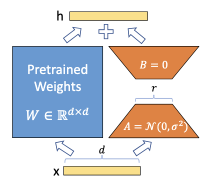
To ensure training of the adaptation starts from the pre-trained model (i.e., $\Delta W = 0$), we must initialize the product $BA$ to zero. The standard solution is to set one matrix to zero (typically $B$) and initialize the other with values sampled from a random distribution. But why not initialize the matrices the other way around? Or avoid zeroing out one matrix by initializing both such that they are orthogonal (and their product is zero)^[3]?

In this post, we compare the training dynamics and generalization capabilities of three distinct paradigms: 1. Standard (Init[A]): $A\sim \mathcal{N}, B=0$ 2. Reversed (Init[B]): $A=0, B\sim \mathcal{N}$ 3. Orthogonal: $A\neq 0, B\neq 0, A \perp B$ such that $BA=0$

Background: Initialization variance¶

To prevent exploding or vanishing gradients, standard initialization methods (such as Glorot ^[4] or Kaiming ^[5]) scale the variance of weight inversely with the input dimension ($d_\text{in}$):

Standard:

$$ \begin{align*} \sigma^2_A &\propto \frac{1}{d_\text{in}} \\ B &= 0 \end{align*} $$

As models get wider (larger $d_\text{in}$), the variance of $A$ decreases. This more conservative initialization seems to perfectly counterbalance the model's high dimensionality.

For matrix $B\in \mathbb{R}^{d_\text{out}\times r}$ the "input dimension" is the LoRA rank $r$. Crucially, $r$ is fixed and thus does not change when the model gets wider:

Reversed:

$$ \begin{align*} A &= 0 \\ \sigma^2_B &\propto \frac{1}{r} \end{align*} $$

This scheme injects variance into the weights scaling with $1/r$. Since $r \ll d_\text{in}$, the term $1/r$ is relatively large. This results in a dangerously high variance regardless of model size. This forces the model into a fragile state where it cannot tolerate the higher learning rates required for optimal convergence.

The difference becomes more intuitive if we think of LoRA not just as a product of two low-rank matrices that is applied to the initial weight matrix, but instead as a parallel path with a downscale and upscale projection. $A$ represents the downscaling from $d_\text{in}$ to $r$, and $B$ the upscaling from $r$ to $d_\text{out}$. Since $r\ll d_\text{in}$, initialization for both matrices looks quite different.

The Hypotheses¶

This post aims to test the following two hypotheses.

The Variance Scaling Hypothesis (Standard vs. Reversed)¶

Hayou et al.^[1] suggest that the standard initialization is superior to the reversed version due to how variance scales with width.

We test this claim empirically with a modern LLM, new dataset, over a range of seven different learning rates and with four runs per configuration (with varying seeds).

The Diversity Hypothesis (Standard vs. Orthogonal)¶

One downside of setting $B=0$ is that a large portion of the initial weights is zero and thus $A$ receives zero gradients for the first and relatively small gradients for the early steps, and the update for $B$ depends on the random initialization of $A$. Orthogonal initialization attempts to fix this. By initializing $A$ and $B$ with orthogonal matrices from a QR decomposition or permutations of unit vectors, we ensure $BA=0$ while keeping the weights non-zero. This theoretically allows gradients to flow through both matrices immediately.

Experimental Setup¶

We conduct a sweep of experiments using Qwen2.5-1.5B on the no_robots dataset across seven learning rates ($1\times 10^{-4}$ to $1\times 10^{-2}$). We average four runs per configuration using different seeds to obtain reliable results.

For each learning rate we test five initializations: - Standard: $A\sim \text{Kaiming}, B=0$ - Reversed: $A=0, B\sim \text{Kaiming}$ - Orthogonal Eye: $Q=I$, rows split between $A$ and $B$ - Orthogonal QR (const): Random orthogonal $Q$, rows split between $A$ and $B$, constant variance ^[3] - Orthogonal QR (matched): Random orthogonal $Q$, rows split between $A$ and $B$, variance matched to Kaiming init

Results¶

The results show that the values for the learning rate $\eta$ can be categorized into three distinct groups.

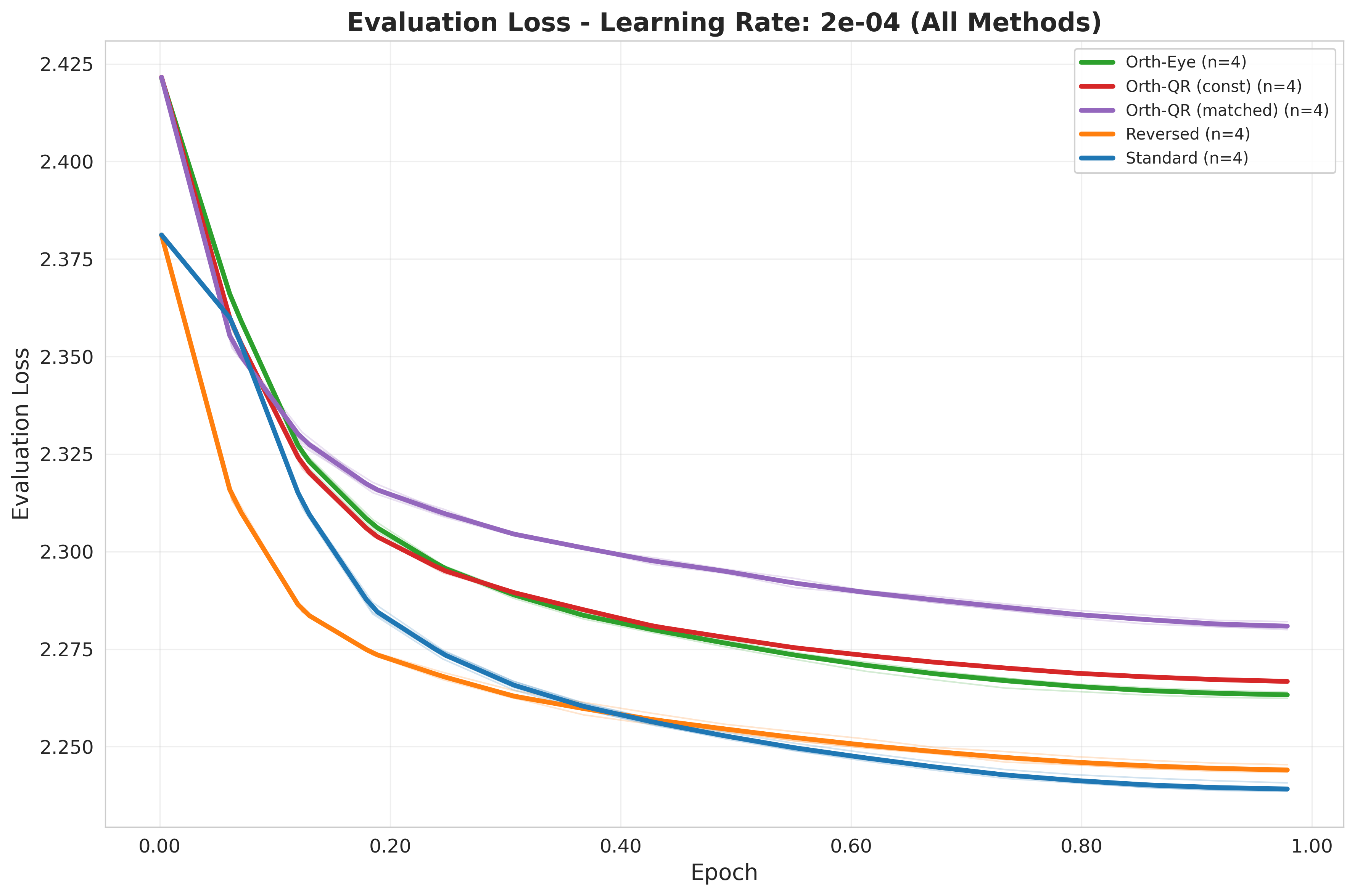
Group 1: Safe, small learning rate ($\eta = 2\times 10^{-4}$)¶

At conservative learning rates, initialization plays a minor role. All methods converge reliably. Interestingly, Reversed showed a slight advantage over Standard here, but neither reaches their optimal loss in this learning rate group.

$\eta$	Standard	Reversed	Ortho (Eye)	Ortho QR (Const)	Ortho QR (Match)
$1\times 10^{-4}$	$2.2576$	$2.2513$	$2.2801$	$2.2802$	$2.2874$
$2\times 10^{-4}$	$2.2391$	$2.2440$	$2.2633$	$2.2667$	$2.2809$

Here is a relative comparison of each result with Standard as baseline: | $\eta$ | Standard | Reversed | Ortho (Eye) | Ortho QR (Const) | Ortho QR (Match) | | :--- | :--- | :--- | :--- | :--- | :--- | | $1\times 10^{-4}$ | Baseline | $-0.28\%$ | $+0.99\%$ | $+1.00\%$ | $+1.32\%$ | | $2\times 10^{-4}$ | Baseline | $+0.22\%$ | $+1.08\%$ | $+1.23\%$ | $+1.86\%$ |

Group 2: A gap starts to form ($5\times 10^{-4} \leq \eta \leq 2 \times 10^{-3}$)¶

Increasing the learning rate accelerates training (up to a limit) and, in the case of Standard, improves generalization. This is the regime where the best evaluation losses are found, with Standard clearly dominating.

The more sophisticated Orthogonal methods fail to outperform the standard baseline. In fact, introducing non-zero weights in both matrices seems to hinder optimization compared to keeping one matrix at zero.

$\eta$	Standard	Reversed	Ortho (Eye)	Ortho QR (Const)	Ortho QR (Match)
$5\times 10^{-4}$	$2.2228$	$2.2461$	$2.2558$	$2.2611$	$2.2827$
$1\times 10^{-3}$	$2.2178$	$2.2607$	$2.2592$	$2.2700$	$2.3014$
$2\times 10^{-3}$	$2.2173$	$2.2898$	$2.2721$	$2.2925$	$7.0413$

Here again the relative comparison against Standard: | $\eta$ | Standard | Reversed | Ortho (Eye) | Ortho QR (Const) | Ortho QR (Match) | | :--- | :--- | :--- | :--- | :--- | :--- | | $5\times 10^{-4}$ | Baseline | $+1.05\%$ | $+1.49\%$ | $+1.72\%$ | $+2.70\%$ | | $1\times 10^{-3}$ | Baseline | $+1.93\%$ | $+1.87\%$ | $+2.35\%$ | $+3.77\%$ | | $2\times 10^{-3}$ | Baseline | $+3.27\%$ | $+2.47\%$ | $+3.39\%$ | $+217\%$ |

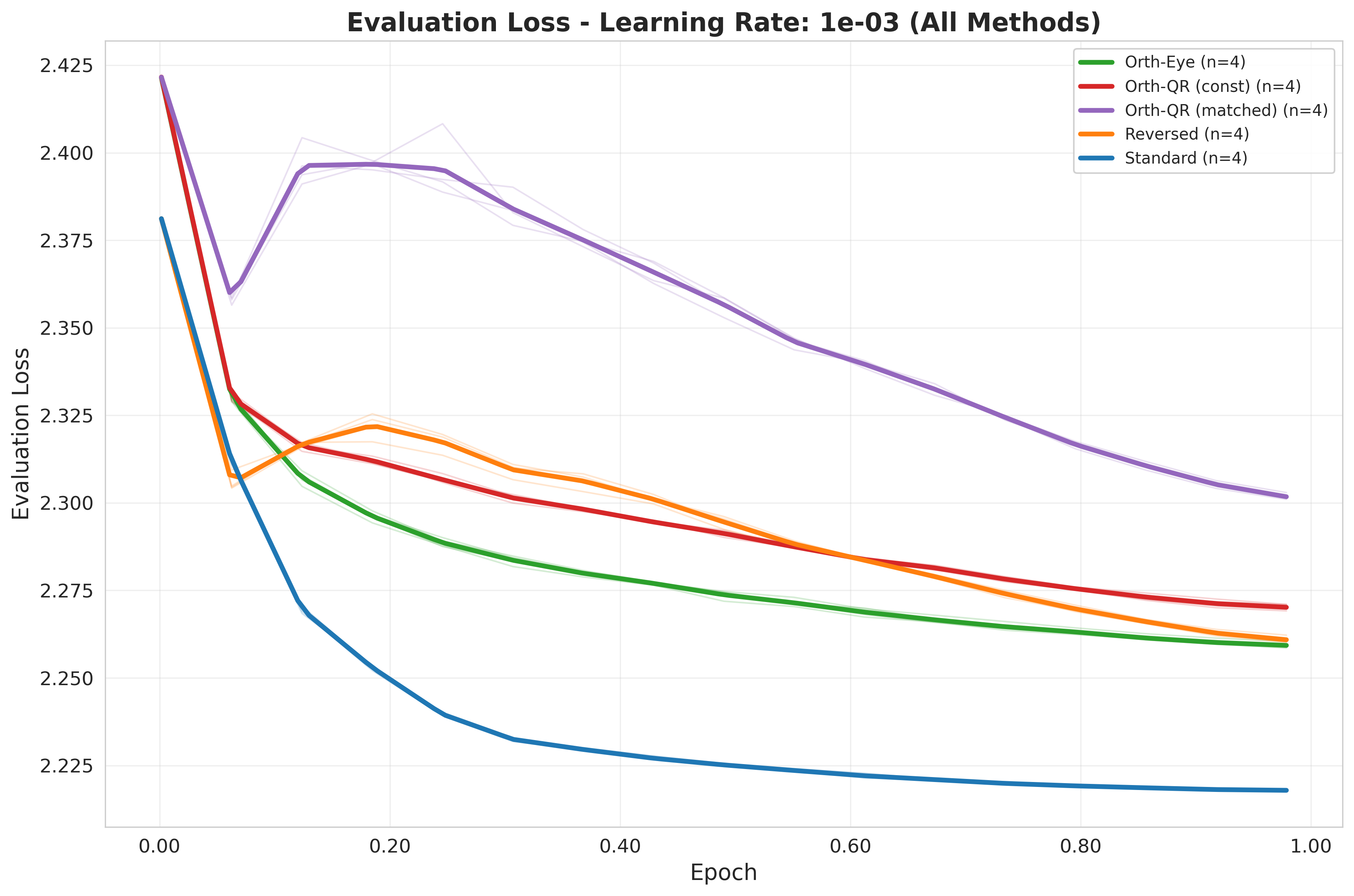
Tracking the evaluation loss reveals instability in the learning process of Reversed and the Orthogonal methods, especially when compared to the textbook-like, smooth descent of Standard.

Lastly, let's see what happens if we further increase the learning rate.

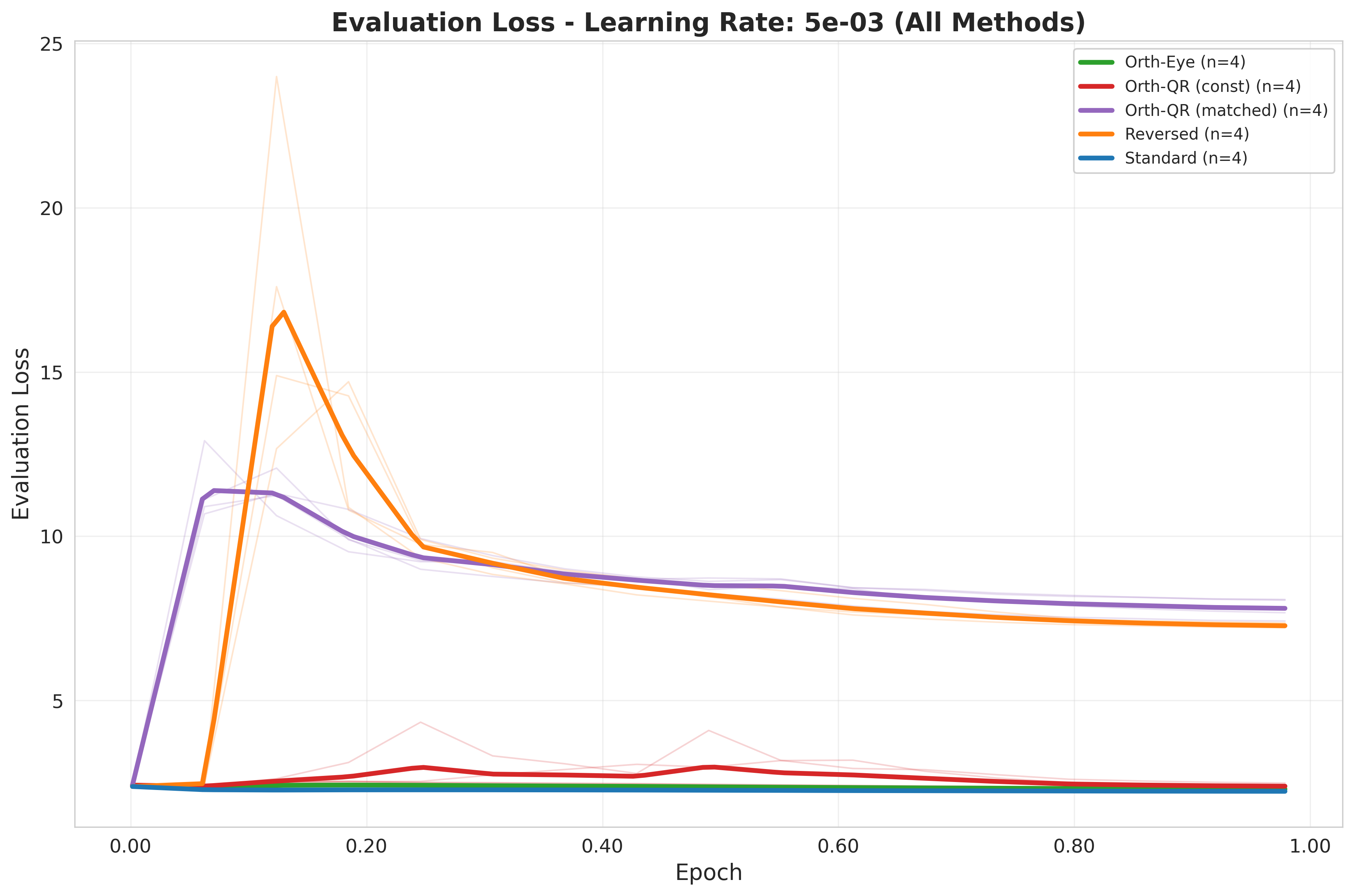
Group 3: The Stability Cliff ($\eta \geq 5\times 10^{-3}$)¶

At even higher learning rates, the robustness of the initialization schemes is tested:

• Standard: Achieves a strong evaluation loss for $5\times 10^{-3}$. Increasing the learning rate further leads to instability even for this initialization scheme.
• Reversed: As predicted by the variance scaling hypothesis, this scheme leads to exploding loss due to instability.
• Orthogonal QR: Interestingly, the Kaiming matched variance scheme is less stable in this setup and explodes right away. The constant variance stays stable for one more learning rate increase, until it finally also becomes unstable.
• Orthogonal Eye: Similar to constant Orthogonal QR, it remains stable (at a higher value than Standard) and only gets unstable in the last experiment.

$\eta$	Standard	Reversed	Ortho (Eye)	Ortho QR (Const)	Ortho QR (Match)
$5\times 10^{-3}$	$2.2348$	$7.2726$	$2.3011$	$2.3891$	$7.8028$
$1\times 10^{-2}$	$9.3169$	$7.7805$	$7.4645$	$7.1409$	$7.8530$

$\eta$	Standard	Reversed	Ortho (Eye)	Ortho QR (Const)	Ortho QR (Match)
$5\times 10^{-3}$	Baseline	$+225\%$	$+2.96\%$	$+6.90\%$	$+249\%$
$1\times 10^{-2}$	Baseline	$-16.49\%$	$-19.88\%$	$-23.35\%$	$-15.71\%$

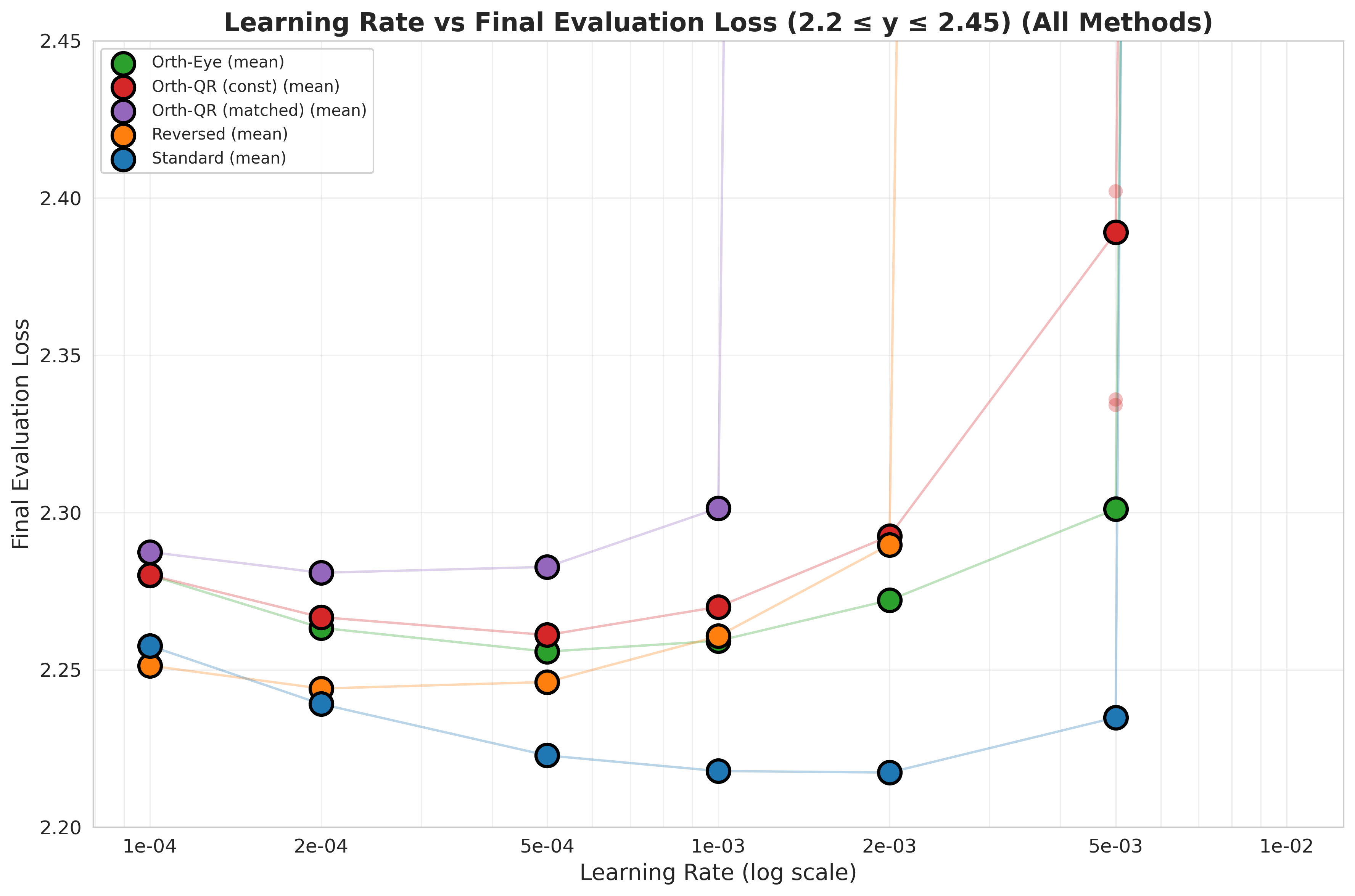
Overview¶

We recreate and extend the plot from ^[1] which shows the final evaluation loss for different initialization schemes and learning rates:

The instability outliers for higher learning rates make it impossible to see differences for smaller learning rates, so here is a zoomed-in version:

Analysis¶

Our results suggest that strictly zeroing one matrix (Standard) is better than ensuring the zero-product via orthogonality ($B\perp A$). It seems that the restriction of having the first update steps of $B$ constrained by the random projection $A$, while $A$ is not or only slowly changed, does not hurt but helps the optimization process.

When both $A$ and $B$ are non-zero (Orthogonal), the optimization landscape is more complex from step 0. The optimizer must adjust two sets of active weights simultaneously. This appears to make the optimization task harder and less stable.

The failure of Orthogonal QR (Matched) at high learning rates is particularly telling. This method attempted to combine the "diversity" of orthogonal vectors with the "scaling" of Kaiming initialization. Its catastrophic divergence, alongside Reverse, confirms that variance injection into the low-rank bottleneck is dangerous.

Conclusion¶

Sometimes simple methods just work, but still validate your choices.

While the Orthogonal initialization theoretically appears to be a powerful way to enable better optimization steps from the outset, empirically, it does not yield performance benefits and actually hinders stability.

When thinking about whether to initialize $A$ or $B$ randomly and set the other one to zero, you might not immediately spot the difference in variance. Therefore, and since these experiments are rather fast, it is a good recommendation to just try it out.

The code is available here.