nanochat's gpt.py
Annotated nanochat
Roughly a month ago Andrej Karpathy published nanochat, calling it "The best ChatGPT that $100 can buy". [1]
I immediately took a look at it, since Karpathy's resources are usually of exceptional quality. And that was also the case for nanochat. For me, who recently started to work on LLMs/VLMs, this was a great opportunity to dive into deep details with a clean, minimal code base.
To force myself to work through every line and try to understand them, I started this post. I hope it helps others as much as it helped me.
And with that, let's start with the line-by-line walktrough of nanochat/gpt.py.
Configuration
@dataclass
class GPTConfig:
    sequence_len: int = 1024
    vocab_size: int = 50304
    n_layer: int = 12
    n_head: int = 6 # number of query heads
    n_kv_head: int = 6 # number of key/value heads (MQA)
    n_embd: int = 768
This is a convenient method of keeping track of the parameters of the LLM and accessing them via class attributes instead of e.g., dictionary keys (which would be more prone to misspelling and less supported by LSPs/autocomplete). We will discuss the effect of the individual values when they are used, but we already see a few characteristics of the default configuration:
sequence_len = 1024: Compared to modern language models that is a rather short maximal sequence length. E.g., GPT-5 has a context length of 400k, and Gemini 2.5 even of 1 million, but training those models also cost slightly more than 100$vocab_size = 50304: We talked about that when we saw the tokenizer.- There are the same values for query and key/value heads, so we would have a (standard) multi-head attention (MHA). However, having separate variables for them allows us to easily configure a nowadays commonly used multi-query attention (MQA) mechanism.
Components of Transformer
def norm(x):
    # Purely functional rmsnorm with no learnable params
    return F.rms_norm(x, (x.size(-1),))
This is a simple wrapper around the torch.nn.functional.rms_norm function, that simplifies the code later on.
It is a deviation from most other Transformer implementations that commonly use torch.nn.LayerNorm.
Unlike the standard torch.nn.LayerNorm, this version is non-parameterized, so it has no learnable scale (gamma) or shift (beta) parameters. This simplifies the model and saves a small number of parameters. [2]
def apply_rotary_emb(x, cos, sin):
    assert x.ndim == 4  # multihead attention
    d = x.shape[3] // 2
    x1, x2 = x[..., :d], x[..., d:] # split up last time into two halves
    y1 = x1 * cos + x2 * sin # rotate pairs of dims
    y2 = x1 * (-sin) + x2 * cos
    out = torch.cat([y1, y2], 3) # re-assemble
    out = out.to(x.dtype) # ensure input/output dtypes match
    return out
Now it gets more interesting. If you are familiar with the standard Transformer architecture you probably remember that before we pass the inputs to the encoder/decoder blocks we add a positional encoding to them. That is required since Transformers are permutation-invariant, i.e., they are not aware of the ordering of tokens. Well, that is not how modern LLMs do it anymore, because there are some disadvantages to that (blog post is in work). To keep it short, the traditional absolute positonal encoding has the disadvantage that a model has to figure out that tokens at position 1 and 6 have the same distance between them as tokens at position 22 and 27. While they are quite capable of doing a good job at it (with enough data), they do not learn that equivariance perfectly and have to spend considerable model capacity on this simple task. So the modern way of providing positional information to a Transformer is to rotate token vectors according to their position (and rotate each position by a different frequency, similar to positional encoding). This has the advantage that the dot product between two tokens (as performed for key-query matching) is a function of the values of the two tokens and the difference of their positions:
$$ \langle f_q (x_m, m), f_k(x_n, n) \rangle = g(x_m, x_n, m - n) $$
From [3].
What we see here is the implementation of the rotation of an input tensor x. The other two arguments cos and sin are precomputed values for specific frequencies and positions (we will see their values later).
In the second line we see a check that only passes if the input has four dimensions (batch, head, sequence, features). Especiallly during development that can catch crucial errors and potentially save hours of debugging.
Next a variable d is introduced that just corresponds to half of the feature dimension and shortens the next line.
The we split the input along the feature axis right in the middle to get two equally big tensors x1 and x2.
Now we can perform the rotation: lines 5 and 6 correspond to a 2D vector rotation:
$$ \begin{pmatrix} y_1 \\ y_2 \end{pmatrix} = \begin{pmatrix} \cos\theta & \sin\theta \\ -\sin\theta & \cos\theta \end{pmatrix} \begin{pmatrix} x_1 \\ x_2 \end{pmatrix} $$
Finally in lines 7 and 8 the two results y1 and y2 are combined back to have the same shape as the input x and their datatype is set to be consistent.
What is interesting in this function is, that the implementation does not follow RoPE as it was proposed in the paper (always two neighboring values form a 2D vector, e.g., positions 0 and 1, 2 and 3, ...), but instead values from the first half of the vector form a pair with values from the second half (e.g., 0 and d, 1 and d+1, ...).
This is computationally easier to perform (we just need to split the matrix in half, instead of interleaving it), and seems to make no difference to the effectiveness of positional awareness.
def repeat_kv(x, n_rep):
    """torch.repeat_interleave(x, dim=1, repeats=n_rep)"""
    if n_rep == 1:
        return x
    bs, n_kv_heads, slen, head_dim = x.shape
    return (
        x[:, :, None, :, :]
        .expand(bs, n_kv_heads, n_rep, slen, head_dim)
        .reshape(bs, n_kv_heads * n_rep, slen, head_dim)
    )
Again, a simple helper function that will simplify the code later on. It just repeats key or value tensors, such that we can use them in Grouped-Query Attention [4] (K and V dimensions are smaller than Q in that case and we need to repeat them so the dimensions can broadcast during the attention calculation. But let's see line by line:
Arguments of the function are the tensor to be repeated x and the number of repetitions n_rep. If n_rep is equal ot one we can simply return the input x as nothing has to be done.
If n_rep is larger than one, we first get the named dimensions of x (for convenience).
The actual interleaved repetition is then performed directly in the return part: [:, :, None, :, :] adds a new dimension in the middle (new shape is (bs, n_kv_heads, 1, slen, head_dim)), along which we then repeat the tensor with .expand.
Using expand instead of repeat_interleave is a significant optimization: repeat_interleave would create a new tensor, copying the data n_rep times, whereas expand just creates a new view on the original data without consuming extra memory. The subsequent attention calculation can work directly with this view.
Finally we call .reshape to collapse the newly introduced dimension and merges it with n_kv_heads. This leaves us with the desired interleaved repetitions of the input tensor x.
class CausalSelfAttention(nn.Module):
    def __init__(self, config, layer_idx):
        super().__init__()
        self.layer_idx = layer_idx
        self.n_head = config.n_head
        self.n_kv_head = config.n_kv_head
        self.n_embd = config.n_embd
        self.head_dim = self.n_embd // self.n_head
        assert self.n_embd % self.n_head == 0
        assert self.n_kv_head <= self.n_head and self.n_head % self.n_kv_head == 0
        self.c_q = nn.Linear(self.n_embd, self.n_head * self.head_dim, bias=False)
        self.c_k = nn.Linear(self.n_embd, self.n_kv_head * self.head_dim, bias=False)
        self.c_v = nn.Linear(self.n_embd, self.n_kv_head * self.head_dim, bias=False)
        self.c_proj = nn.Linear(self.n_embd, self.n_embd, bias=False)
The next class is split into multiple parts to better follow the code step by step.
We start with the initialization method of the CausalSelfAttention class, that sets up all required parts for the forward pass based on the config (of type GPTConfig).
All relevant configuration values (n_head, n_kv_head and n_embed) are stored as class variables, along-side the other argument of the function layer_idx (required for kv caching later).
After that we compute the dimension of each attention head (head_dim) and ensure that the embedding dimension n_embed is divisible by n_head and n_head is a multiple of n_kv_head.
Based on the values for key/value and query heads, we set up the projection matrices that will transform the inputs into keys, values and queries (c_q, c_k, c_v). All three of them have the same input dimension n_embed, since they all project the same input. Their second dimension depends on the values of n_head (for queries) and n_kv_heads (for keys and values).
Note that the output dimension of the query projection is the same as the input dimension, since we calculated head_dim as the division of n_embed and n_head. Following the asserts we can also already infer that the output dimension of the key and value projections is either the same as that of the query projection or smaller (in which case we need repeat_interleave later for the multiplication).
Slowly all parts come together. To see how they interact with each other, we need to look at the forward method.
    def forward(self, x, cos_sin, kv_cache):
        B, T, C = x.size()

        # Project the input to get queries, keys, and values
        q = self.c_q(x).view(B, T, self.n_head, self.head_dim)
        k = self.c_k(x).view(B, T, self.n_kv_head, self.head_dim)
        v = self.c_v(x).view(B, T, self.n_kv_head, self.head_dim)

        # Apply Rotary Embeddings to queries and keys to get relative positional encoding
        cos, sin = cos_sin
        q, k = apply_rotary_emb(q, cos, sin), apply_rotary_emb(k, cos, sin) # QK rotary embedding
        q, k = norm(q), norm(k) # QK norm
        q, k, v = q.transpose(1, 2), k.transpose(1, 2), v.transpose(1, 2) # make head be batch dim, i.e. (B, T, H, D) -> (B, H, T, D)

        # Apply KV cache: insert current k,v into cache, get the full view so far
        if kv_cache is not None:
            k, v = kv_cache.insert_kv(self.layer_idx, k, v)
        Tq = q.size(2) # number of queries in this forward pass
        Tk = k.size(2) # number of keys/values in total (in the cache + current forward pass)

        # Apply MQA: replicate the key/value heads for each query head
        nrep = self.n_head // self.n_kv_head
        k, v = repeat_kv(k, nrep), repeat_kv(v, nrep)

        # Attention: queries attend to keys/values autoregressively. A few cases to handle:
        if kv_cache is None or Tq == Tk:
            # During training (no KV cache), attend as usual with causal attention
            # And even if there is KV cache, we can still use this simple version when Tq == Tk
            y = F.scaled_dot_product_attention(q, k, v, is_causal=True)
        elif Tq == 1:
            # During inference but with a single query in this forward pass:
            # The query has to attend to all the keys/values in the cache
            y = F.scaled_dot_product_attention(q, k, v, is_causal=False)
        else:
            # During inference AND we have a chunk of queries in this forward pass:
            # First, each query attends to all the cached keys/values (i.e. full prefix)
            attn_mask = torch.zeros((Tq, Tk), dtype=torch.bool, device=q.device) # True = keep, False = mask
            prefix_len = Tk - Tq
            if prefix_len > 0: # can't be negative but could be zero
                attn_mask[:, :prefix_len] = True
            # Then, causal attention within this chunk
            attn_mask[:, prefix_len:] = torch.tril(torch.ones((Tq, Tq), dtype=torch.bool, device=q.device))
            y = F.scaled_dot_product_attention(q, k, v, attn_mask=attn_mask)

        # Re-assemble the heads side by side and project back to residual stream
        y = y.transpose(1, 2).contiguous().view(B, T, -1)
        y = self.c_proj(y)
        return y
This is the largest code block so far, but also contains a lot of comments. The relevant code parts are surprisingly straightforward. Again, we start with the arguments passed to the method, which in this case are an input x (note that it batched, so one input does not imply one text sample), precomputed cosine and sine values cos_sin and a kv_cache that stores already computed key/value values
B, T and C correspond to the dimensions of the input (batch, sequence length / time, and feature dimension). The first important part of this method is then the projection of x into queries q, keys k and values v using the previously initialized projection matrices. In the same lines where we do the projection, we also directly perform a .view operation, that similarly to .expand early changes the view of the tensor to give us a new shape (in this case splitting the feature dimension into separate heads each with head_dim features) without actually moving the underlying data around.
Now that we have the keys, queries and values, we can apply the previously discussed rotational postional encoding to the keys and queries, using the function apply_rotary_emb and the provided precomputed values for cosine and sine of different frequencies.
After the rotations we normalize queries and keys and finally change the order of the dimensions of all three tensors to have T and D (sequence length and feature dimensions) as the last two, such that they are used for the following matrix multiplications.
The reason for QK-normalization is to avoid that the attention logits explode: Given the attention formula
$$ \text{Attention}(Q, K, V) = \text{softmax}\left(\frac{QK^T}{\sqrt{d_k}}\right)V $$
without a normalization (or clipping) of $Q$ and $K$ we might end up with very large products of $QK^T$. [5]
The computation of keys and values is expensive and has to be repeated many times due to the autoregressive nature of LLMs, so it's common to store those values in a kv_cache. While that significantly increases our memory consumption it simultaneously decreases the time of new token generation by much.
We will see what happens in the kv_cache when we call insert_kv later, when we reach the implementation of it.
Generally you can think of the kv-cache to be a dictionary with some size limit, that automatically deletes old entries whenit reaches it maximum storage capacity.
Before we come to the actual attention operation, we store the numbers of queries Tq and the number of key/values Tk, as we need them in a second. Furthermore, we need to call repeat_kv to change the dimension of keys and values such that they match those of the queries.
Applying the attention mechanism differs slightly depending on the availability of the kv_cache (only during inference) and the number of queries in case of an available kv-cache. Let's look at all three cases and see, how and why they differ:
- Case 1 No kv-cache (training phase) or during prefill of inference (before autoregressive generation): During training we have the benefit of knowing already the full sequence we want to predict and we can use this fact to perform a prediction for the next token at every position simultaneously. This greatly increases efficiency and is possible by restricting the attention mechanism to only look back. E.g., for predicting the fifth token we want the attention to only use the first four tokens, while for the sixth token we want to look also at the fifth. This restriction of not looking back is implemented with a causal masking matrix that is a binary lower triangular matrix that is multiplied with the attention scores. We enable this causal masking by setting
is_causal=True.
- Case 2 There is just a single query (simple next token prediction during inference). We call the same function as in the first case, but this time disable the causal masking with
is_causal=False. - Case 3 Multiple queries during inference: This is a slightly advanced case, which could be used for speculative decoding. We basically provide a potential next token sequence and validate that. The implementation of it is a combination of case 1 and 2, since we need full attention for all previous kv values (like in case 2), but a causal masking for the newly predicted tokens (like in case 1). For that reason we have to manually construct the attention mask with
Truefor the context (up untilprefix_len) and a triangular lower part (tril) afterwards. This matrix is then passed to the dot product calculation.
Finally as a last step we just need reverse the transposing we did earlier to then combine the heads back into one dimension (.view(B, T, -1)). That tensor is then passed through the final output projection c_proj.
class MLP(nn.Module):
    def __init__(self, config):
        super().__init__()
        self.c_fc = nn.Linear(config.n_embd, 4 * config.n_embd, bias=False)
        self.c_proj = nn.Linear(4 * config.n_embd, config.n_embd, bias=False)

    def forward(self, x):
        x = self.c_fc(x)
        x = F.relu(x).square()
        x = self.c_proj(x)
        return x
This class is small and simple, yet it has arguably one of the most important parts of the final model. Sure, attention gets a lot attribution of the success of LLMs, but the weights of the MLP (multi-layer percepton) layers contribute a lot to the final performance of the LLM and also make up the largest portion of trainable parameters.
nanochat keeps the MLP class simple; in the initialization are just two linear layers introduced and in the forward pass they are sequentially applied to the input with a non-linearity inbetween (square relu).
But lets have a quick look at what there is happening in detail. The first linear layer (c_fc) is also called up-projection, since it is a mapping from a n_embed dimensional input to a four times as large output. Then a squared relu actvation function (y = (max(0, x))**2) [6] is applied to introduce some non-linearity, before we down-project the tensor back to its input dimensionality with c_proj.
class Block(nn.Module):
    def __init__(self, config, layer_idx):
        super().__init__()
        self.attn = CausalSelfAttention(config, layer_idx)
        self.mlp = MLP(config)

    def forward(self, x, cos_sin, kv_cache):
        x2 = x + self.attn(norm(x), cos_sin, kv_cache)
        out = x2 + self.mlp(norm(x2))
        return out
Note that I modified the variable names in the forward method. In `nanochat` all `x`, `x2` and `out` are named `x`, which would have made the explanations somewhat more difficult.
The next class combines some of the things we have so far to build a Block. Parts of the Block are a CausalSelfAttention layer as well as a MLP layer.
The forward method is slightly more interesting, but should look familiar if you know the basic Transformer decoder block structure: To get an intermediate representation x2 we add to the input x the output of the CausalSelfAttention of the normalized input x. So we have here a residual connection around the normalization and attention. Similarly we have a residual connection around another normalization and the MLP block, to get to the output representation out.
This way of applying the normalization is called Pre-Norm, which nowadays seems to be preferred over Post-Norm (as proposed in the original Transformer paper), since it is more stable especially in bigger models. [7]
The other parameter cos_sin and kv_cached are just passed to the CausalSelfAttention layer, since they are required there as we saw.
Putting everything together
class GPT(nn.Module):
    def __init__(self, config):
        super().__init__()
        self.config = config
        self.transformer = nn.ModuleDict({
            "wte": nn.Embedding(config.vocab_size, config.n_embd),
            "h": nn.ModuleList([Block(config, layer_idx) for layer_idx in range(config.n_layer)]),
        })
        self.lm_head = nn.Linear(config.n_embd, config.vocab_size, bias=False)
        # To support meta device initialization, we init the rotary embeddings here, but it's fake
        # As for rotary_seq_len, these rotary embeddings are pretty small/cheap in memory,
        # so let's just over-compute them, but assert fail if we ever reach that amount.
        # In the future we can dynamically grow the cache, for now it's fine.
        self.rotary_seq_len = config.sequence_len * 10 # 10X over-compute should be enough, TODO make nicer?
        head_dim = config.n_embd // config.n_head
        cos, sin = self._precompute_rotary_embeddings(self.rotary_seq_len, head_dim)
        self.register_buffer("cos", cos, persistent=False) # persistent=False means it's not saved to the checkpoint
        self.register_buffer("sin", sin, persistent=False)
        # Cast the embeddings from fp32 to bf16: optim can tolerate it and it saves memory: both in the model and the activations
        self.transformer.wte.to(dtype=torch.bfloat16)
And with that we finally arrived at the main class of this file, GPT. This class will combine everything we implemented so far and is the final model that can be trained and used.
In the __init__ method we first store the config object for later internal use. Next we create all required components of our model, namely a nn.Embedding layer and a list of Blocks. The list of Blocks and the dict storing both the list and the nn.Embedding are packed inside a nn.ModuleList resp. nn.ModuleDict. This ensures that pytorch is aware of the parameters and can provide them to the optimizer or move the to a device with .to(). Forgetting this is a common error for pytorch beginners and usually results in either an error message or a model not training.
Additionally, we also need to add a lm_head, that is a Linear layer that maps the final token representations to logits for the next token.
You might have seen in other GPT implementations that the weights of the embedding layer wte and the lm_head (un-embedding layer) are tied (i.e., they share the same weight matrix). This is a popular technique (weight-tying) to save parameters. nanochat keeps them separate, which is a simpler design and also a valid choice.
Next the values of sin and cos for the rotational encoding are precomputed. Since they do not require much space, they are directly precomputed for 10x the sequence length that is used during training. This means during inference we can use a larger context than we trained on (this is another benefit of RoPE: since the model sees positional differences rather than absolute positions, it can generalize to a larger context with similar performance).
After precomputing the values, they are stored as buffers with register_buffer. This ensures that they are moved to the correct device, but are not seen as learnable parameters (so pytorch does not need to compute gradients). Since their computation is very fast, we do not need to store them in model checkpoint files, which is achieved with persistent=False.
Finally, the memory footprint of the embedding layer is reduces by transformingit's values to bfloat16.
    def init_weights(self):
        self.apply(self._init_weights)
        # zero out classifier weights
        torch.nn.init.zeros_(self.lm_head.weight)
        # zero out c_proj weights in all blocks
        for block in self.transformer.h:
            torch.nn.init.zeros_(block.mlp.c_proj.weight)
            torch.nn.init.zeros_(block.attn.c_proj.weight)
        # init the rotary embeddings
        head_dim = self.config.n_embd // self.config.n_head
        cos, sin = self._precompute_rotary_embeddings(self.rotary_seq_len, head_dim)
        self.cos, self.sin = cos, sin

    def _init_weights(self, module):
        if isinstance(module, nn.Linear):
            # https://arxiv.org/pdf/2310.17813
            fan_out = module.weight.size(0)
            fan_in = module.weight.size(1)
            std = 1.0 / math.sqrt(fan_in) * min(1.0, math.sqrt(fan_out / fan_in))
            torch.nn.init.normal_(module.weight, mean=0.0, std=std)
            if module.bias is not None:
                torch.nn.init.zeros_(module.bias)
        elif isinstance(module, nn.Embedding):
            torch.nn.init.normal_(module.weight, mean=0.0, std=1.0)
The initalization of weights is split into two methods init_weights and _init_weights. The reason for that is to make use of torch.nn.Module.apply, which applies a initialization method efficiently to all parameters. Since we need to overwrite some of that initializations the self.apply call with _init_weights is wrapped in the method init_weights together with the desired overwrites.
First, we look at how all parameters are initialized in _init_weights: Following [8] all weights of linear layers are randomly initialized with a zero-mean gaussian distribution with a standard deviation $\sigma = \frac{1}{\sqrt{\text{fan\_in}}} \min \left( 1, \sqrt{\frac{\text{fan\_out}}{\text{fan\_in}}} \right)$. Biases of those layers, if activated, are initialized with zero.
In contrast to that the embedding layer is randomly initialized with a zero-mean gaussian with a standard deviation of $1$.
We already discussed, that those initializations are performed using self.apply as a first step in init_weights to then overwrite some of the values at particular positions.
One of those locations is the lm_head, which is the final layer for the next token prediction and all its weights are set to zero.[^1]
Other weight matrices that are set to zero are the final projection matrices in both the attention and MLP layers.
Initializing the final layer of a residual block to zero makes the entire block act as an identity function at the start of training. This can significantly stabilize training for deep networks. Similarly, zero-initing the lm_head ensures that the model outputs zero logits at initialization, which corresponds to a uniform probability distribution over the vocabulary as an unbiased starting point (it would be interesting to see some ablations on whether this improves the training).
Finally this method calls _precompute_rotary_embeddings (which we will analyze next) to precompute the values that we pass around as cos and sin for the rotary encoding.
    # TODO: bump base theta more, e.g. 100K is more common more recently
    def _precompute_rotary_embeddings(self, seq_len, head_dim, base=10000, device=None):
        # autodetect the device from model embeddings
        if device is None:
            device = self.transformer.wte.weight.device
        # stride the channels
        channel_range = torch.arange(0, head_dim, 2, dtype=torch.float32, device=device)
        inv_freq = 1.0 / (base ** (channel_range / head_dim))
        # stride the time steps
        t = torch.arange(seq_len, dtype=torch.float32, device=device)
        # calculate the rotation frequencies at each (time, channel) pair
        freqs = torch.outer(t, inv_freq)
        cos, sin = freqs.cos(), freqs.sin()
        cos, sin = cos.bfloat16(), sin.bfloat16() # keep them in bfloat16
        cos, sin = cos[None, :, None, :], sin[None, :, None, :] # add batch and head dims for later broadcasting
        return cos, sin
Now we get to the part whose result was used quite some times already. In _precompute_rotary_embeddings we precompute the values for cos and sin that are later used to rotate keys and queries. Since the rotation angles stay the same and do not take up too much space, we do the computation once and store the results.
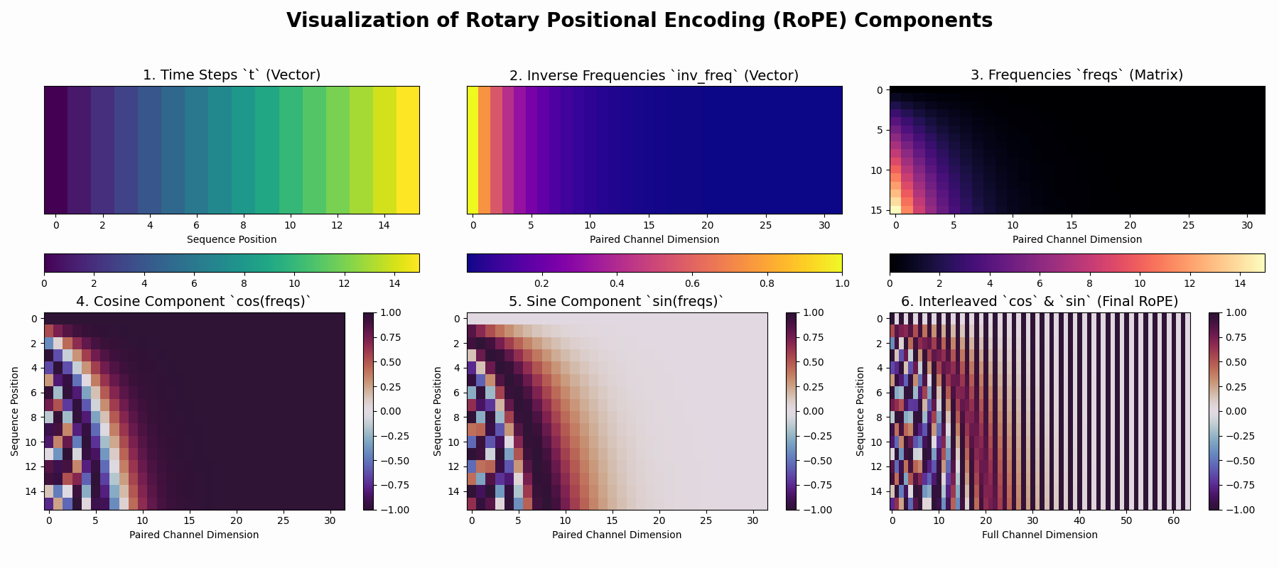
First, this method detects the used device, if it is not provided as argument. Next, it computes the rotation parameters accoring to the RoPE formula. Each line is quite straightforward and only introduces a single variable or transformation, but it can still help to visualize the content of the relevant variables for a smaller example.
Click here to see the code that generated the figure
import matplotlib.colors as mcolors
import matplotlib.pyplot as plt
import torch

torch.manual_seed(42)

head_dim = 64
base = 10000.0
seq_len = 16

# RoPE Precomputation (just like in nanochat)
channel_range = torch.arange(0, head_dim, 2, dtype=torch.float32)
inv_freq = 1.0 / (base ** (channel_range / head_dim))
t = torch.arange(seq_len, dtype=torch.float32)
freqs = torch.outer(t, inv_freq)
cos = freqs.cos()
sin = freqs.sin()

fig, axs = plt.subplots(2, 3, figsize=(18, 8), facecolor="#FDFDFD")
fig.suptitle(
    "Visualization of Rotary Positional Encoding (RoPE) Components",
    fontsize=20,
    weight="bold",
)

# consistent color map and normalization for cos/sin
norm = mcolors.Normalize(vmin=-1, vmax=1)
cmap = "twilight_shifted"

# Plot 1: Time Steps `t`
im1 = axs[0, 0].imshow(t.unsqueeze(0), cmap="viridis", aspect="auto")
axs[0, 0].set_title("1. Time Steps `t` (Vector)", fontsize=14)
axs[0, 0].set_xlabel("Sequence Position")
axs[0, 0].set_yticks([])
fig.colorbar(im1, ax=axs[0, 0], orientation="horizontal", pad=0.2)

# Plot 2: Inverse Frequencies `inv_freq`
im2 = axs[0, 1].imshow(inv_freq.unsqueeze(0), cmap="plasma", aspect="auto")
axs[0, 1].set_title("2. Inverse Frequencies `inv_freq` (Vector)", fontsize=14)
axs[0, 1].set_xlabel("Paired Channel Dimension")
axs[0, 1].set_yticks([])
fig.colorbar(im2, ax=axs[0, 1], orientation="horizontal", pad=0.2)

# Plot 3: Frequencies `freqs`
im3 = axs[0, 2].imshow(freqs, cmap="magma", aspect="auto")
axs[0, 2].set_title("3. Frequencies `freqs` (Matrix)", fontsize=14)
axs[0, 2].set_xlabel("Paired Channel Dimension")
# axs[0, 2].set_ylabel("Sequence Position") # shared with the plots below
fig.colorbar(im3, ax=axs[0, 2], orientation="horizontal", pad=0.2)

# Plot 4: Cosine of Frequencies
im4 = axs[1, 0].imshow(cos, cmap=cmap, norm=norm, aspect="auto")
axs[1, 0].set_title("4. Cosine Component `cos(freqs)`", fontsize=14)
axs[1, 0].set_xlabel("Paired Channel Dimension")
axs[1, 0].set_ylabel("Sequence Position")
fig.colorbar(im4, ax=axs[1, 0])

# Plot 5: Sine of Frequencies
im5 = axs[1, 1].imshow(sin, cmap=cmap, norm=norm, aspect="auto")
axs[1, 1].set_title("5. Sine Component `sin(freqs)`", fontsize=14)
axs[1, 1].set_xlabel("Paired Channel Dimension")
axs[1, 1].set_ylabel("Sequence Position")
fig.colorbar(im5, ax=axs[1, 1])

# Plot 6: Combined View
final_rope = torch.stack((cos, sin), dim=-1).flatten(start_dim=-2)
im6 = axs[1, 2].imshow(final_rope, cmap=cmap, norm=norm, aspect="auto")
axs[1, 2].set_title("6. Interleaved `cos` & `sin` (Final RoPE)", fontsize=14)
axs[1, 2].set_xlabel("Full Channel Dimension")
axs[1, 2].set_ylabel("Sequence Position")
fig.colorbar(im6, ax=axs[1, 2])


plt.tight_layout()
plt.show()
Keep in mind RoPE actually rotates queries and keys, in contrast to absolute positional encodings where some vector is added to the input tokens. So the bottom row of sin and cos is not added to the vectors, but instead used for the rotation. Still it shows that this seemingly simple formula creates a complex pattern, that follows some structure.
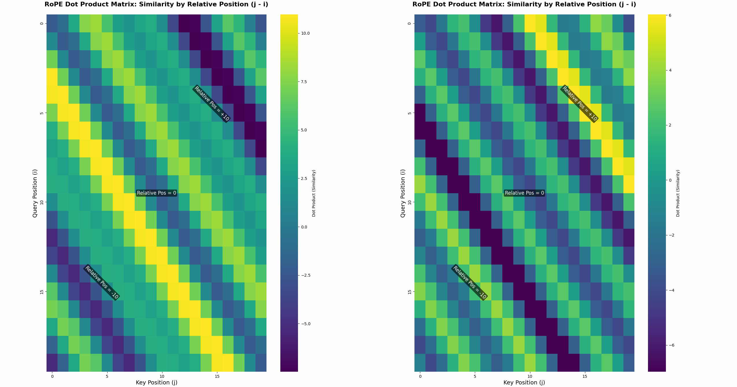
To highlight the relative positional part see the next plot:
Click here to see the code that generated the figure
import matplotlib.pyplot as plt
import numpy as np
import seaborn as sns
import torch

torch.manual_seed(42)

head_dim = 32
base = 10000.0
seq_len = 20

# RoPE Precomputation (just like in nanochat)
channel_range = torch.arange(0, head_dim, 2, dtype=torch.float32)
inv_freq = 1.0 / (base ** (channel_range / head_dim))
t = torch.arange(seq_len, dtype=torch.float32)
freqs = torch.outer(t, inv_freq)
cos_lookup = freqs.cos()
sin_lookup = freqs.sin()


# again: just like nanochat (and many others)
def apply_rope(vector, position_idx, cos_l, sin_l):
    vector_pairs = vector.float().reshape(-1, 2)
    cos_vals = cos_l[position_idx]
    sin_vals = sin_l[position_idx]

    rotated_v0 = vector_pairs[:, 0] * cos_vals - vector_pairs[:, 1] * sin_vals
    rotated_v1 = vector_pairs[:, 0] * sin_vals + vector_pairs[:, 1] * cos_vals

    rotated_vector = torch.stack((rotated_v0, rotated_v1), dim=-1).flatten()
    return rotated_vector


def plot_dot_products(q, k, axes=None):
    dot_product_matrix = np.zeros((seq_len, seq_len))

    # Calculate pairwise dot products
    for i in range(seq_len):  # Query positions
        q_vec_rotated = apply_rope(q, i, cos_lookup, sin_lookup)
        for j in range(seq_len):  # Key positions
            k_vec_rotated = apply_rope(k, j, cos_lookup, sin_lookup)
            dot_product_matrix[i, j] = torch.dot(q_vec_rotated, k_vec_rotated).item()

    if axes is None:
        fig, axes = plt.subplots(1, 1, figsize=(10, 8), facecolor="#FDFDFD")

    plot_heatmap(
        axes,
        dot_product_matrix,
        seq_len,
        "RoPE Dot Product Matrix: Similarity by Relative Position (j - i)",
    )


def plot_heatmap(ax, dot_product_matrix, seq_len, title):
    sns.heatmap(
        dot_product_matrix,
        ax=ax,
        cmap="viridis",
        annot=False,
        fmt=".2f",
        cbar_kws={"label": "Dot Product (Similarity)"},
        xticklabels=5,
        yticklabels=5,
    )

    ax.set_xlabel("Key Position (j)", fontsize=14)
    ax.set_ylabel("Query Position (i)", fontsize=14)
    ax.set_title(
        title,
        fontsize=16,
        weight="bold",
        pad=20,
    )
    ax.tick_params(axis="x", labelsize=10)
    ax.tick_params(axis="y", labelsize=10)

    # Annotations
    ax.text(
        seq_len * 0.5,
        seq_len * 0.5,
        "Relative Pos = 0",
        color="white",
        ha="center",
        va="center",
        fontsize=12,
        bbox=dict(
            facecolor="black", alpha=0.6, edgecolor="none", boxstyle="round,pad=0.2"
        ),
    )

    ax.text(
        seq_len * 0.75,
        seq_len * 0.25,
        "Relative Pos = +10",
        color="white",
        ha="center",
        va="center",
        fontsize=12,
        bbox=dict(
            facecolor="black", alpha=0.6, edgecolor="none", boxstyle="round,pad=0.2"
        ),
        rotation=-45,
    )

    ax.text(
        seq_len * 0.25,
        seq_len * 0.75,
        "Relative Pos = -10",
        color="white",
        ha="center",
        va="center",
        fontsize=12,
        bbox=dict(
            facecolor="black", alpha=0.6, edgecolor="none", boxstyle="round,pad=0.2"
        ),
        rotation=-45,
    )


if __name__ == "__main__":
    fig, ax = plt.subplots(1, 2, figsize=(10, 16), facecolor="#FDFDFD")

    base_q = torch.randn(head_dim)  # A base vector for q
    base_k = torch.randn(head_dim)  # A base vector for k
    plot_dot_products(base_q, base_k, ax[0])

    base_q = torch.randn(head_dim)  # A base vector for q
    base_k = torch.randn(head_dim)  # A base vector for k
    plot_dot_products(base_q, base_k, ax[1])

    plt.tight_layout()
    plt.show()
This figure shows the same thing twice just with two randomly initialized vectors, so we can focus on the left part: We have two vectors q and k that are multiplied and in the plot we see the result of their rotated versions.
What this figure shows is that the dot product actually does stay the same for same position differences. That is the whole point of RoPE and what makes it so powerful.
    def get_device(self):
        return self.transformer.wte.weight.device

    def estimate_flops(self):
        """ Return the estimated FLOPs per token for the model. Ref: https://arxiv.org/abs/2204.02311 """
        nparams = sum(p.numel() for p in self.parameters())
        nparams_embedding = self.transformer.wte.weight.numel()
        l, h, q, t = self.config.n_layer, self.config.n_head, self.config.n_embd // self.config.n_head, self.config.sequence_len
        num_flops_per_token = 6 * (nparams - nparams_embedding) + 12 * l * h * q * t
        return num_flops_per_token
Next we have some helper functions, that are less relevant. get_device has a pretty self explaining method name and so does estimate_flops. For the FLOPs (Floating Point Operations) estimation the formula from the famous Palm paper [9] (Appendix B), that specifices the number of FLOPs as six times the number of parameters nparams (of which Karpathy excluded the parameters for the embedding layer nparams_embedding), plus 12 times the product of number of layers l, the number of heads h, head dimensions q and sequence length t.
If you want to learn more about calculating in FLOPs in Transformers you should definetly check out this seminal (series of) blog posts[10]: How to scale your model
    def setup_optimizers(self, unembedding_lr=0.004, embedding_lr=0.2, matrix_lr=0.02, weight_decay=0.0):
        model_dim = self.config.n_embd
        ddp, rank, local_rank, world_size = get_dist_info()
        # Separate out all parameters into 3 groups (matrix, embedding, lm_head)
        matrix_params = list(self.transformer.h.parameters())
        embedding_params = list(self.transformer.wte.parameters())
        lm_head_params = list(self.lm_head.parameters())
        assert len(list(self.parameters())) == len(matrix_params) + len(embedding_params) + len(lm_head_params)
        # Create the AdamW optimizer for the embedding and lm_head
        # Scale the LR for the AdamW parameters by ∝1/√dmodel (having tuned the LRs for 768 dim model)
        dmodel_lr_scale = (model_dim / 768) ** -0.5
        if rank == 0:
            print(f"Scaling the LR for the AdamW parameters ∝1/√({model_dim}/768) = {dmodel_lr_scale:.6f}")
        adam_groups = [
            dict(params=lm_head_params, lr=unembedding_lr * dmodel_lr_scale),
            dict(params=embedding_params, lr=embedding_lr * dmodel_lr_scale),
        ]
        adamw_kwargs = dict(betas=(0.8, 0.95), eps=1e-10, weight_decay=weight_decay)
        AdamWFactory = DistAdamW if ddp else partial(torch.optim.AdamW, fused=True)
        adamw_optimizer = AdamWFactory(adam_groups, **adamw_kwargs)
        # Create the Muon optimizer for the linear layers
        muon_kwargs = dict(lr=matrix_lr, momentum=0.95)
        MuonFactory = DistMuon if ddp else Muon
        muon_optimizer = MuonFactory(matrix_params, **muon_kwargs)
        # Combine them the two optimizers into one list
        optimizers = [adamw_optimizer, muon_optimizer]
        for opt in optimizers:
            for group in opt.param_groups:
                group["initial_lr"] = group["lr"]
        return optimizers
Yes, you saw that right, there is a setup_optimizers method in our model class. At least I was caught by surprise, since usually my optimizer's setup takes place before the training loop in the main code. But in this case it makes sense, because the optimizers initalization (yes, plural) is highly customized to the model and especially in a setup with multiple model architectures it quickly could become messy if we handle all initalizations at the same place.
So let's have a look: First we already get a hint for the number of parameter-groups that we differentiate, namely embedding, unembedding (or commonly refered to as lm_head) and matrix (basically the rest).
The first two lines of the method are used to store some information about the model (model_dim) and GPU environment that are used later. Next, we gather all parameters, separate them in the aforementioned three groups and make sure that these three groups represent the whole parameter set.
Then we introduce a scaling factor for the learning rate based on the model dimension. It basically scales down the learning rate for larger models, according to μP (μParametrization) [11]: The goal of μP is to parameterize a model so that its optimal hyperparameters (like learning rate) remain stable as the model's width or depth are scaled.
We can then scale the provided learning rates for the embedding and lm_head parameters by this factor and together with the constant values for betas=(0.8, 0.95) and the provided weight_decay initialize an AdamW optimizer (how it is provided by the AdamWFactory is part of another file and thus blog post).
For the matrix_params set we initialize a Muon optimizer [12], which is a somewhat new, but very well performing optimization algorithm, that by now is used quite commonly in LLMs. And according to Twitter, this way of using separate optimizers is "pretty well known at this point".
But you also find a good explanation, at least providing some intuition on why this works so well:
The common high level intuition is that embedding is a lookup table and you don't want interaction between rows. Muon is by definition taking the full matrix to make the update, AdamW is a parameter wise update. It's the same intuition for why we don't do weight decay on…
— elie (@eliebakouch) October 14, 2025
Finally the learning rate lr for each optimizer and parameter group is stored in initial_lr, which could be useful later when a scheduler comes into play.
    def forward(self, idx, targets=None, kv_cache=None, loss_reduction='mean'):
        B, T = idx.size()

        # Grab the rotary embeddings for the current sequence length (they are of shape (1, seq_len, 1, head_dim))
        assert T <= self.cos.size(1), f"Sequence length grew beyond the rotary embeddings cache: {T} > {self.cos.size(1)}"
        assert idx.device == self.cos.device, f"Rotary embeddings and idx are on different devices: {idx.device} != {self.cos.device}"
        assert self.cos.dtype == torch.bfloat16, "Rotary embeddings must be in bfloat16"
        # if kv cache exists, we need to offset the rotary embeddings to the current position in the cache
        T0 = 0 if kv_cache is None else kv_cache.get_pos()
        cos_sin = self.cos[:, T0:T0+T], self.sin[:, T0:T0+T] # truncate cache to current sequence length

        # Forward the trunk of the Transformer
        x = self.transformer.wte(idx)
        x = norm(x)
        for block in self.transformer.h:
            x = block(x, cos_sin, kv_cache)
        x = norm(x)

        # Forward the lm_head (compute logits)
        softcap = 15
        if targets is not None:
            # training mode: compute and return the loss
            # TODO: experiment with Liger Kernels / chunked cross-entropy etc.
            logits = self.lm_head(x)
            logits = softcap * torch.tanh(logits / softcap) # logits softcap
            logits = logits.float() # use tf32/fp32 for logits
            loss = F.cross_entropy(logits.view(-1, logits.size(-1)), targets.view(-1), ignore_index=-1, reduction=loss_reduction)
            return loss
        else:
            # inference mode: compute and return the logits
            logits = self.lm_head(x)
            logits = softcap * torch.tanh(logits / softcap) # logits softcap
            return logits
The forward method is again quite straightforward and mostly builds upon our previous implementations. B and T store the dimensions of the input indices with B being the batch size and T the (maximum, possible padded) sequence length. After that, we assert a few things about the precomputed sine and cosine values for the rotarty encoding, such as that it is at least as long as the input, on the same device as the input and has the datatype bfloat16.
Next we need to account for the length of a possible kv-cache, since that offsets the starting position of the input ids idx. If the kv_cache is provided, our first token index in idx is not at position 0 of the whole sequence, so we slice the precomputed sine and cosine values accordingly.
After that we can pass the input idx first through the embedding layer wte, then normalize the tokens, pass it through each block with our sliced cos_sin values and the kv_cache. The output tokens from the transformer blocks are again normalized, before we proceed with the prediction head lm_head.
We did not talk about the method arguments yet, but already seen how idx (the inputs) and kv_cache are used. The other two arguments targets and loss_reduction are optional and only provided during training, and we will see how they are used now.
Depending on whether targets is provided, we detect if we are in training mode (targets is not None, we need to predict the next token distribution and calculate the loss with respect to the provided targets) or inference mode (targets is None, we just want to generate the next token). Besides the loss calculation, both paths are the same, so it would have been possible to pull the pass through lm_head and the softcapped logit calculation outside of the if-else. But now let's have a more close look at softcapping logits:
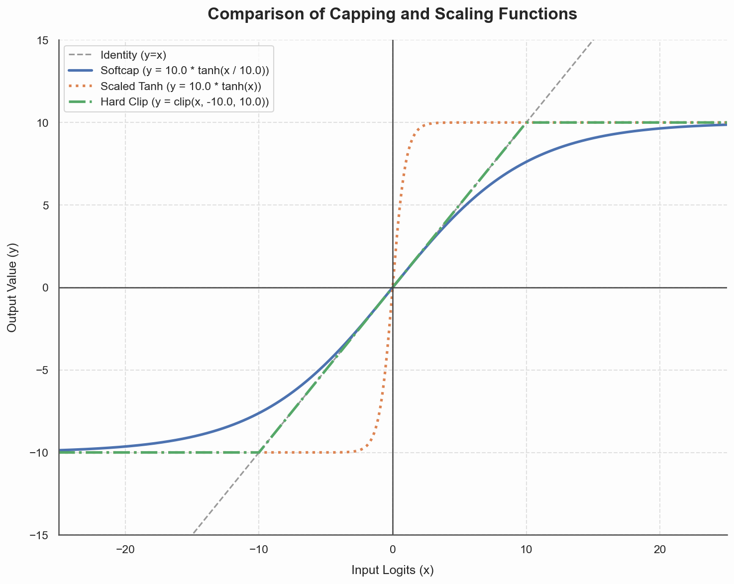
Softcapping is a solution to avoid too large logits, but instead of clipping them (which would destroy the gradients), it uses a scaled tanh for it. [13]
As you can see below, this really looks like a softer version of clipping the values, and due to the scaling of the logits before applying tanh it has a similar slope and is not as steep as just a scaled tanh.
Click here to see the code that generated the figure
import matplotlib.pyplot as plt
import seaborn as sns
import torch

logits = torch.arange(-50.0, 50.0, 0.01, dtype=torch.float32)
bound = 10.0


def softcap(x):
    return bound * torch.tanh(x / bound)


softcapped_logits = softcap(logits)
scaled_tanh_logits = bound * torch.tanh(logits)
capped_logits = torch.clip(logits, -bound, bound)

sns.set_theme(
    style="whitegrid",
    rc={
        "grid.linestyle": "--",
        "grid.color": "#e0e0e0",
        "axes.facecolor": "#FDFDFD",
        "figure.facecolor": "#FDFDFD",
        "axes.edgecolor": "#555555",
    },
)

fig, ax = plt.subplots(1, 1, figsize=(10, 8))

ax.plot(
    logits,
    logits,
    label="Identity (y=x)",
    linestyle="--",
    color="grey",
    alpha=0.8,
    linewidth=1.5,
)
ax.plot(
    logits,
    softcapped_logits,
    label=f"Softcap (y = {bound} * tanh(x / {bound}))",
    linewidth=2.5,
)
ax.plot(
    logits,
    scaled_tanh_logits,
    label=f"Scaled Tanh (y = {bound} * tanh(x))",
    linewidth=2.5,
    linestyle=":",
)
ax.plot(
    logits,
    capped_logits,
    label=f"Hard Clip (y = clip(x, -{bound}, {bound}))",
    linewidth=2.5,
    linestyle="-.",
)


ax.axhline(0, color="#444444", linewidth=1.2, linestyle="-")
ax.axvline(0, color="#444444", linewidth=1.2, linestyle="-")

# Set plot limits to focus on the interesting area where functions differ
ax.set_xlim(-25, 25)
ax.set_ylim(-15, 15)

ax.set_xlabel("Input Logits (x)", fontsize=12, labelpad=10)
ax.set_ylabel("Output Value (y)", fontsize=12, labelpad=10)
ax.set_title(
    "Comparison of Capping and Scaling Functions", fontsize=16, pad=20, weight="bold"
)

ax.legend(loc="upper left", frameon=True, shadow=False, fontsize=11)

sns.despine(ax=ax, offset=0)

plt.tight_layout()
plt.show()
In case of detected training (targets are not None), we finish the forward pass by calculating the cross-entropy loss between predicted and target logits and return this loss. How the loss values are reduced over the batch dimension (e.g., average, sum, keep as list), is determined by the other method argument loss_reduction.
Note that during inference we return the predicted next token logits not just for the last token, but for the whole sequence. This will be relevant in the next method.
And with that we have reached the final code block of this file, the containing the generate method.
    @torch.inference_mode()
    def generate(self, tokens, max_tokens, temperature=1.0, top_k=None, seed=42):
        """
        Naive autoregressive streaming inference.
        To make it super simple, let's assume:
        - batch size is 1
        - ids and the yielded tokens are simple Python lists and ints
        """
        assert isinstance(tokens, list)
        device = self.get_device()
        rng = None
        if temperature > 0:
            rng = torch.Generator(device=device)
            rng.manual_seed(seed)
        ids = torch.tensor([tokens], dtype=torch.long, device=device) # add batch dim
        for _ in range(max_tokens):
            logits = self.forward(ids) # (B, T, vocab_size)
            logits = logits[:, -1, :] # (B, vocab_size)
            if top_k is not None:
                v, _ = torch.topk(logits, min(top_k, logits.size(-1)))
                logits[logits < v[:, [-1]]] = -float('Inf')
            if temperature > 0:
                logits = logits / temperature
                probs = F.softmax(logits, dim=-1)
                next_ids = torch.multinomial(probs, num_samples=1, generator=rng)
            else:
                next_ids = torch.argmax(logits, dim=-1, keepdim=True)
            ids = torch.cat((ids, next_ids), dim=1)
            token = next_ids.item()
            yield token
generate has the torch.inference_mode() decorator, which just as torch.no_grad() disables gradient computation for this part. inference_mode is slightly more restricted, as it does also not allow any tensors created in this context to participate in autograd operations. [^2]
As the comments say, this method is very simple and rather basic, it does not even use the kv-cache. We will see how to use the kv-cache during autoregressive generation in nanochat/engine.py (future post).
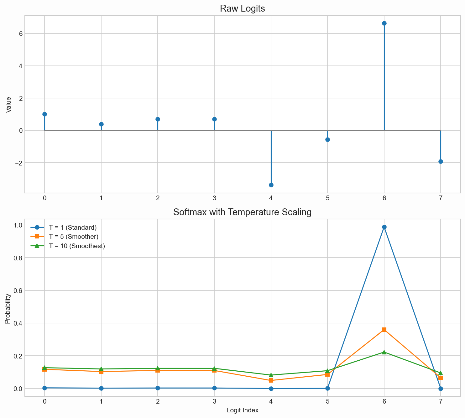
The method requires two arguments, the input tokens which should be continued tokens and max_tokens as an upper bound of tokens to generate. Additionally it accepts a temperature which controls the sampling of next tokens (lower temperature chooses most likely tokens, higher temperature gets closer towards uniform sampling, see figure below).
Click here to see the code that generated the figure
import matplotlib.pyplot as plt
import torch

torch.manual_seed(42)

plt.style.use('seaborn-v0_8-whitegrid')

logit_dim = 8
x = list(range(logit_dim))

logits = torch.randn(logit_dim) * 3

fig, axs = plt.subplots(2, 1, figsize=(10, 9), facecolor="#FDFDFD")

(markers, stemlines, baseline) = axs[0].stem(x, logits, label="Logits")
plt.setp(baseline, 'color', 'grey', 'linewidth', 1)
axs[0].set_title("Raw Logits", fontsize=14)
axs[0].set_ylabel("Value")

axs[1].plot(x, torch.softmax(logits, dim=-1),
            label="T = 1 (Standard)", marker='o')
axs[1].plot(x, torch.softmax(logits / 5, dim=-1),
            label="T = 5 (Smoother)", marker='s')
axs[1].plot(x, torch.softmax(logits / 10, dim=-1),
            label="T = 10 (Smoothest)", marker='^')

axs[1].set_title("Softmax with Temperature Scaling", fontsize=14)
axs[1].set_ylabel("Probability")
axs[1].set_xlabel("Logit Index")
axs[1].legend()

for ax in axs:
    ax.set_xticks(x)

plt.tight_layout()
plt.show()
The method itself is again not very complex, since it is mainly a wrapper around the forward pass with a sampling from the predicted next token distribution.
First, it is checked that tokens is just a list, the device is stored in a local variable and a reproducible random number generator rng is initialized if temperature > 0 (for temperature == 0 we would have a greedy version). After that the list of input tokens is wrapped in an additional dimension and then transformed into a torch.tensor, which now looks like a batched input with a single sample.
Passing this tensor to self.forward lets the model predict the probability distribution for the next token at every position. Because we are only interested in the last position, we can slice it along the T dimension and get a single probability distribution (since B == 1).
Next we select the next token based on this probability distribution and the provided arguments:
First we reduce the number of tokens to sample from, if top_k is not None. In that case we select all token probabilities that are smaller than the k-largest and set them to negative infinity.
Then we either select the most likely token in a greedy way (if temperature == 0) by choosing the token with the highest predicted probability, or sample from the predicted distribution with the provided temperature.
Finally, the newly selected token is appended to our tokens tensor, such that the next iteration continues the generation in an autoregressive way, and also yielded back to the caller.
Final thoughts
That's it! This was the first file of nanochat, in which the model architecture was defined and useful methods like forward and generate were introduced.
I learnt a lot while trying to understand overy line of the implementation:
- Benefits of RoPE and how it is implemented
- Normalizing queries and keys to keep attention logits from growing too large and thus improve stability
- That different optimizers are used for different sets of the parameters
- How to soft-cap logits to keep them bound but also keep gradients
It was a lot of work, but I feel like it was worth it and it was also fun. Andrej's style of structuring the code makes it possible to quickly understand all parts and how they interact with each other.
The plan is to do a similar line-by-line exploration of the other (relevant) files. If you have any feedback, or found any errors, feel free to reach out!
BibTeX
@misc{nanochat-2025,
  author = {Alexander Weers},
  title = {nanochat's gpt.py},
  url = {https://aweers.de/blog/2025/nanochat/},
}
References
-
nanochat: The best ChatGPT that \$100 can buy
2025 ↩ -
Root mean square layer normalization
Advances in neural information processing systems, 2019 ↩ -
Roformer: Enhanced transformer with rotary position embedding
Neurocomputing, 2024 ↩ -
GQA: Training Generalized Multi-Query Transformer Models from Multi-Head Checkpoints
Proceedings of the 2023 Conference on Empirical Methods in Natural Language Processing, 2023 ↩ -
Scaling Vision Transformers to 22 Billion Parameters
Proceedings of the 40th International Conference on Machine Learning, 2023 ↩ -
Searching for efficient transformers for language modeling
Advances in neural information processing systems, 2021 ↩ -
On layer normalization in the transformer architecture
International conference on machine learning, 2020 ↩ -
A spectral condition for feature learning
arXiv preprint arXiv:2310.17813, 2023 ↩ -
Palm: Scaling language modeling with pathways
Journal of Machine Learning Research, 2023 ↩ -
How to Scale Your Model
2025 ↩ -
Tensor programs v: Tuning large neural networks via zero-shot hyperparameter transfer
arXiv preprint arXiv:2203.03466, 2022 ↩ -
Muon: An optimizer for hidden layers in neural networks
2024 ↩ -
Gemma 2: Improving open language models at a practical size
arXiv preprint arXiv:2408.00118, 2024 ↩