Denser rewards, nearly free: contrastive potential shaping
TL;DR: This post explores the effect of adding paragraph-level credit assignment to GRPO-style RL by tracking how each reasoning prefix changes a scorer's relative likelihood of correct and incorrect answers from the rollout group. On Countdown with Qwen3-0.6B, a frozen scorer improves pass@1 after 30 steps from 54.7 to 60.7 across three runs compared to the GRPO-style baseline. The advantage vanishes for longer training runs (60.4 baseline vs 59.4 shaped at step 240), but a moving scorer reaches higher step-240 performance (63.9).
After a target-span KV-cache optimization in vLLM, the frozen-scorer runs take 97 minutes instead of 216 minutes (before optimization), so the overhead of the denser learning signal is minimal (baseline takes 93 minutes).
The credit assignment problem
After the initial success and strong performance of PPO for reinforcement learning for LLMs [1][2][3], the introduction of GRPO and its demonstration in the training of DeepSeek-R1 led to a large movement away from value models as they exist in PPO. Group-relative policy gradient methods such as GRPO avoid training and serving a separate critic model. Given the huge size of LLMs, this is an important systems advantage. The main assumption for group-level methods is that whatever led to a correct result is probably a good way to solve the task. The trade-off is that a dense learning signal (PPO provides a signal for each token) is lost and replaced by one outcome signal for an entire generated sequence.
This leads to a poor description of many reasoning traces. Most contain both correct and incorrect attempts, wandering, restating the question and current steps, backtracking, and educated guessing. The policy gradient nevertheless reinforces or penalizes every token using the same outcome-level signal.
This creates three practical problems:
- efficiency/sparse feedback: sampling rollouts is expensive, and for long reasoning traces or complex agentic tasks, it can be very expensive. Still, it produces only one scalar or bit of supervision.
- ambiguity: is it good to restate the question if it sometimes leads to a correct solution and sometimes to an incorrect one? What about other traits that, depending on context, can be a step towards a correct answer or away from it? With one signal per sequence this cannot be separated well.
- slow-start: when no rollout is correct, group-relative methods cannot provide a learning signal, even if some rollouts make progress towards the correct solution.
Related work
The idea of using truncated reasoning traces to estimate progress at intermediate points is an active area of research. This section quickly covers the closest lines of work and what differs in this project.
Process Reward Models
Process reward models (PRMs) grade intermediate reasoning steps [4], which can be used to provide denser feedback. However, they require step-level labels for training, which are costly to acquire and non-trivial to align with progress in solving a task. That also creates an opportunity for exploitation (reward hacking), since the learned reward model might behave in unexpected and undesired ways for some kinds of inputs [5].
Potential-based reward shaping
This project is inspired by potential-based reward shaping (PBRS) [6], which converts a state potential into dense transition rewards while provably leaving the optimal policy unchanged. Classical potentials are task-specific progress measures such as negative distance-to-goal. Ng et al. assume a fixed potential, but Devlin and Kudenko [7] extend the guarantees to time-varying potentials by evaluating each state's potential at the time it is visited. Although this is relevant to the moving scorer introduced later, the guarantees do not directly apply to the advantage shaping used in this post.
This has been applied to LLM training, e.g. via redistributing credit based on the attention map of the reward model [8].
Likelihood as potential
Closest to this project are methods that use the model's belief in the ground-truth answer as the potential. PACR [9] rewards ascending confidence in the ground-truth answer along a trajectory, computed from the policy itself. TIPS [10] shapes dense rewards from the likelihood of the correct answer under a frozen teacher as a static potential. Wang et al. [11] use the step-wise ground-truth likelihood, but keep track of a historical maximum to avoid "pump-and-dump" reward hacking.
Single-reference likelihood potentials have two weaknesses: they are noisy when the answer admits many surface forms, and they conflate semantic progress with stylistic convergence (the likelihood of the correct answer can rise simply because the model settled into the output format).
Sampling-based prefix value
A parallel line of research estimates prefix value by sampling continuations: SPAE [12] probes several short answers after every reasoning step, PPPO [13] samples several continuations from selected prefixes, and VinePPO [14] and Math-Shepherd [15] estimate step value via Monte Carlo rollout success. These give a well-grounded value estimate, at the cost of extra sampling and being blind to sub-threshold progress: after very early steps the correct solution might not yet be sampleable, even though it was a correct reasoning step moving closer towards the correct solution.
Another related project is DenseR [16]: it uses contrast between correct and incorrect rollout representations to redistribute credit at token level. It also leveraged the rollout groups for more than just advantage computation, in this case token-level credit assignment.
This project sits in the likelihood-as-potential line, but replaces single-reference confidence with a contrastive potential over the group's sampled correct and incorrect answers. The contrast is intended to reduce shared stylistic drift and requires no additional generation steps.
Setup
The experiments use prime-rl on two local GPUs, an RTX 3080 and RTX 3090.
prime-rl strikes a nice balance between keeping you informed and not drowning you in log messages, and runs are easy to configure while still allowing enough flexibility.
The task is Sami Khan's Countdown environment, see his blog post for some interesting insights into the task. The setup is pretty simple: given a set of numbers (usually 3-5), the task is to combine them with the arithmetic operations addition, subtraction, multiplication, and division such that their result is equal to a given target.
I like the task: the problem is very simple to understand, solutions are easy to verify, and the difficulty is tunable. Providing three numbers is almost trivial for humans, but six is very hard.
Due to compute constraints, I use Qwen3-0.6B as the base model. It is very small and struggles to solve most three-number problems with a reasonable token cap. This is a good starting point to compare some learning algorithms and their sample-efficiency.
SFT stage
To align the model to a given output format (providing the solution in <solution> ... </solution> tags) and show that these problems are solvable given a limit of 768 tokens, I start with a short supervised fine-tuning (SFT) stage.
As a base dataset I used the response_ws (preferred responses) of asingh15/countdown_tasks_3to4-dpo. It contains short reasoning traces, so it is well suited for our use case.
I did some additional filtering and verification to obtain a high-quality dataset:
- normalizes Unicode ops like ×, ÷, − to ASCII
- strips any trailing = ...
- allows only arithmetic characters
- requires every source number to be used at most once
- evaluates to the target
Then the data is brought into the desired format, with the reasoning in <reasoning> ... </reasoning> tags and the solution in <solution> ... </solution> tags, with no text outside them.
The SFT training is rather straightforward, prime-rl makes it very easy (interesting parts of the configuration below):
SFT config
max_steps = 200

[deployment]
type = "single_node"
num_gpus = 1

[model]
name = "PrimeIntellect/Qwen3-0.6B"
seq_len = 1024

[tokenizer]
name = "PrimeIntellect/Qwen3-0.6B"

[data]
type = "sft"
name = "data/countdown3_ws_sft_clean"
splits = ["train"]
batch_size = 8
seq_len = 1024

[optim]
lr = 1.5e-5

[scheduler]
type = "linear"
warmup_steps = 10
decay_steps = 90
min_lr = 1.5e-6

[renderer]
name = "qwen3"
enable_thinking = true
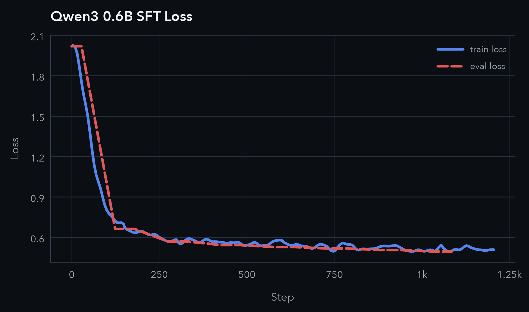
The training takes just half an hour on a single GPU. The loss curves look as boring as desired:
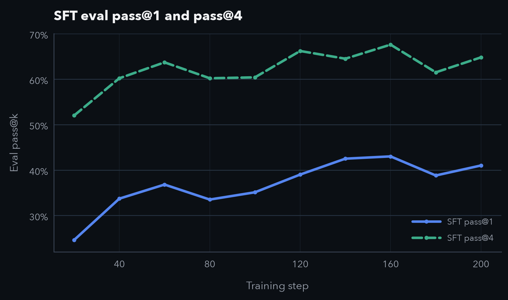
Performance also increased and then plateaued, though this comes mainly from following the required format and thus not being directly rejected by the verifier.
These two examples show the most common scenarios: either the model gets (guesses) the correct solution right away, then double- or triple-checks it and finally submits it, or it tries many approaches without a clear structure, but with very encouraging messages in between ("Finally!", "Got it!").
It is just reproducing patterns it has seen during the (short) SFT stage, but has not learned strategies or step-by-step solving.
RL baseline
To further improve performance, the next step is reinforcement learning on this problem. It is very well suited, since it is
- easily verifiable
- the model has to develop / improve reasoning skills
- we can't provide good off-policy reasoning traces.
prime-rl's default loss is a "DPPO policy-gradient term combined with a KL regularizer":
$$ \mathcal{L}(\theta) = -\,\mathcal{J}_{\text{PG}}(\theta) \;+\; \tau_{KL}\,\mathcal{L}_{KL}(\theta) $$
where the policy-gradient term is
$$ \mathcal{J}_{\text{PG}}(\theta) = \frac{1}{\sum_{j,i} |y_i^{(j)}|} \sum_{j,i,t} \min\!\left(\frac{\pi(y_{i,t}^{(j)}\mid x_j, y_{i, < t}^{(j)})}{\mu(y_{i,t}^{(j)}\mid x_j, y_{i, < t}^{(j)})}, \delta\right) \hat{A}^{(j)}_{i,t} $$
and the KL regularizer penalizes drift between trainer and inference policies via the squared log importance ratio:
$$ \mathcal{L}_{KL}(\theta) = \frac{1}{\sum_{j,i} |y_i^{(j)}|} \sum_{j,i,t} \log^2\!\left(\frac{\pi(y_{i,t}^{(j)}\mid x_j, y_{i, < t}^{(j)})}{\mu(y_{i,t}^{(j)}\mid x_j, y_{i, < t}^{(j)})}\right). $$
I did not change any of its parameters, so these default values are used:
dppo_mask_low=0.2 anddppo_mask_high=0.2adv_tau=1.0kl_tau=1e-3
What I did was a sweep over different learning rates:
| lr | 30-step-pass@1 | 30-step-pass@4 | 60-step-pass@1 | 60-step-pass@4 |
|---|---|---|---|---|
| 1e-5 | 59.9 | 66.6 | 54.0 | 63.5 |
| 5e-6 | 51.8 | 61.7 | 59.4 | 69.3 |
| 2e-6 | 51.9 | 67.4 | 57.9 | 68.9 |
| 4e-7 | 41.3 | 64.5 | 44.0 | 65.2 |
While the picture is less clear after 30 steps, after 60 both 2e-6 and 5e-6 are clearly the best-performing.
Training also seemed relatively stable, as shown by these reward curves:
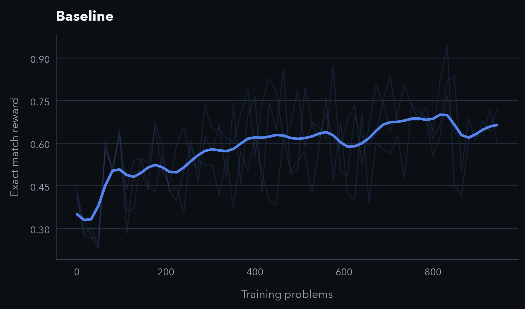
They also show that performance improves significantly after just a few steps before plateauing later at around 70, which is much higher than the post-SFT model.
Some results look promising:
The examples show a clear improvement over the post-SFT checkpoint: it doesn't just guess a solution, but tries different approaches. The first two examples follow a relatively easy recipe, just trying to combine the numbers. That works quickly, since this puzzle is rather simple.
The third example contains a correct idea, but has two flaws in the final solution: it reuses 63 (against the rules), and the * 63 just doesn't make sense.
Another failure case is the fourth example: many different attempts are tried, but they rely too much on the assumption that all numbers have to be used. Interestingly, it still produces a well-formed solution attempt instead of just an endless reasoning chain running into the token limit.
This is our baseline.
Contrastive potential advantage shaping
GRPO (and other outcome-level RL methods) suffer from poor credit assignment, i.e. for each (expensive) rollout you get just one signal (often binary). That is rarely a good description of the reasoning trace, because usually there are good, correct parts that represent steps towards the solution, but also incorrect attempts, wrong conclusions or unsupported guesses. Determining which parts contribute towards finding the solution is non-trivial: to solve a hard math problem it is usually necessary to try a few different approaches, some of which do not lead to the solution. Nevertheless, trying them provides information once an approach is identified as a dead end and the next one can be attempted.
Let's assume we want to move closer towards the correct solution with every step of the reasoning trace. This simple assumption is neither necessarily the true goal, nor fully well-defined without additional choices. What is a step? How do we measure distance towards the solution? What even is "the" solution (there might be many semantically correct ones)?
Inspecting the reasoning traces from the post-SFT checkpoint and the baseline, we take paragraphs as the smallest unit of a step. Sentences would also be a valid choice, but intuitively most individual sentences have rather small influence, so paragraphs seem like the more useful level of abstraction. Formally, we divide a reasoning trace into $|S|$ paragraphs $s_1, \dots, s_{|S|}$, and write $s_{1:n} = (s_1, \dots, s_n)$ for the prefix through the first $n$ paragraphs (with $s_{1:0} = \varnothing$, the empty prefix). A full rollout is then
$$ x,\; s_{1:|S|},\; a $$
where $x$ is the prompt and $a$ is the answer provided in the <solution> tags.
How to measure distance?
This is the most interesting and most impactful question. Given the difficulties already discussed, it is not even clear what a perfect distance measure would look like, let alone a practically implementable one. A reasonable assumption is that we want to gradually increase the likelihood of a correct solution over the course of the reasoning trace. Likelihood estimation is easy with LLMs, it is what they do all the time.
Writing $\ell_\phi(a \mid x, s_{1:n}) = \log p_\phi(a \mid x, s_{1:n})$ for the log-likelihood that a scorer model $\phi$ assigns to an answer string $a$ given a truncated trace, the simplest version scores the single reference answer $a^*$:
$$ \ell_\phi(a^* \mid x, s_{1:n}) $$
Leveraging this likelihood to infer some kind of potential has been examined by several papers, with mixed results [9] [10].
But raw reference-answer likelihood has two problems. First, it is noisy: for multi-token answers, total log-likelihood depends strongly on the answer's length and surface form. This is especially bad when many answers are correct: e.g. for the Countdown task 5 + 11 is a valid way to form 16, but so are 11 + 5, 5+ 11, and (5 + 11).
Second, it mixes semantics with style: the likelihood of a solution can rise simply because the model settled into the output format, not because the reasoning got closer to the answer.
Is that a meaningful step towards solving the problem?
Answer bank
GRPO uses the signal from a group of rollouts to compute a lower-variance advantage, using the group mean as a baseline. We borrow that idea and again use group-level information, this time using all submitted answers in the group. For a set of rollouts we extract all submitted answers and grade them with the verifier, forming the answer bank $\mathcal{B} = \mathcal{B}^{+} \cup \mathcal{B}^{-}$, partitioned into valid/correct answers $\mathcal{B}^{+}$ and invalid/incorrect ones $\mathcal{B}^{-}$ (the ground-truth $a^*$ is optionally added to $\mathcal{B}^{+}$). Rollouts that exceed the token budget contribute nothing to the bank. We need this grading for the main reward anyway, so far there is nothing new. If the group is homogeneous (all submitted answers are correct or all are incorrect), it stays a normal GRPO update (which is empty in that case), since such groups are uninformative and their potential is hard to estimate reliably. [1][1] Consequently, the method in its current form does not address the slow-start case described above, where every rollout is incorrect. It would, however, be trivial to add the provided ground-truth solution to the answer bank for an all-incorrect case to address this. ↩
So assume a group with at least one correct and at least one incorrect submitted solution. This lets us measure a contrastive potential: instead of just the likelihood of the correct answer, we take the gap between the correct and incorrect answers. To aggregate the (multiple) correct or incorrect log-likelihoods into a single number, we use a temperature log-sum-exp,
$$ \mathrm{LSE}_\tau\big(\{z_i\}_{i=1}^{N}\big) = \tau \,\log\!\left(\frac{1}{N}\sum_{i=1}^{N} \exp\!\big(z_i / \tau\big)\right), $$
which interpolates between the maximum ($\tau \to 0^{+}$) and the mean ($\tau \to \infty$) of a set (empirically $\tau = 1$ worked well). The potential after $n$ paragraphs is then the contrast between the two aggregates:
$$ \Phi_n = \mathrm{LSE}_\tau\!\Big(\big\{\ell_\phi(a \mid x, s_{1:n}) : a \in \mathcal{B}^{+}\big\}\Big) \;-\; \mathrm{LSE}_\tau\!\Big(\big\{\ell_\phi(a \mid x, s_{1:n}) : a \in \mathcal{B}^{-}\big\}\Big). $$
Taking a difference can reduce factors shared by correct and incorrect answers, such as settling into a common output format. For example, a paragraph that both explores a new, promising strategy and changes the style of potential solutions (e.g. uses a different order of numbers) should be reinforced. This might not be the case if we measured only the likelihood of a provided ground-truth answer, while in the contrastive formulation some of the stylistic component can cancel between correct and incorrect submitted solutions. The comparison remains sensitive to length differences among answers in the bank, which in this experiment did not lead to any problems and could be fixed.
Finally, we don't use the raw potential directly. We clip it to $\bar{\Phi}_n \in [-5, 5]$ and compute a local difference inspired by the PBRS transition reward:
$$ A_n^{\text{shape}} = \beta\left(\gamma\,\bar{\Phi}_n - \bar{\Phi}_{n-1}\right). $$
The experiments use a scaling factor $\beta=0.1$ and a discount factor $\gamma=0.99$. A discount factor below one (mildly) penalizes remaining at an already high potential for another paragraph, which discourages continuing after the solution becomes clear.
In the implementation $A_n^{\text{shape}}$ is added directly to the advantage of every token in the paragraph $n$ (not divided by paragraph length to avoid a length bias as in vanilla GRPO). This is a deviation from classical PBRS, which adds the potential difference to transition rewards and then computes discounted returns. The policy-invariance guarantee of classical PBRS therefore does not carry over directly.
Putting it together, the algorithm is:
- sample a group of rollouts from the model (as before)
- verify each rollout (as before)
- form the answer bank from the submitted solutions. If the group is homogeneous, fall back to a normal GRPO-style update (which is empty) and continue
- otherwise, split each rollout into paragraphs
- at each paragraph boundary, score the log-likelihood $\ell_\phi$ of every answer in the bank under the scorer $\phi$
- clip the contrastive potential and compute $A_n^{\text{shape}} = \beta(\gamma\bar{\Phi}_n-\bar{\Phi}_{n-1})$
- add $A_n^{\text{shape}}$ to every token advantage in paragraph $n$
One open question is what to use as the scorer $\phi$: the post-SFT checkpoint (a static scorer) or the current policy (a moving scorer)?[2][2] Or a delayed or moving-average model, but that wasn't tested here. ↩
Both have advantages, along very different axes:
- a static scorer provides a stable scoring function. Historically in machine learning, frequently moving targets have been avoided, and where unavoidable they can produce unstable training dynamics and a lot of headaches.
- a moving scorer has the advantage of not requiring a second model to be served during the RL stage. This matters: GRPO's success came partly from removing the value model, so reintroducing a model in memory (even one used only for inference, not training) needs to be justified by a clear performance improvement.
Trying to eliminate as much opportunity for instability as possible, I decided to start with the static scorer.
For my two-GPU setup, that meant the main vLLM server serving the current policy on one GPU (10 GB), and the training script plus the scorer vLLM server on the other (24 GB). That is very tight and required limiting the number of sequences processed in parallel, but it then ran stably.
What does the signal look like?
Before looking at training results, let's have a quick look at the signal provided by the contrastive prefix likelihood. The numbers below are the actual $A_n^{\text{shape}}$ values assigned to every token in each paragraph.
The first example is exactly what we would hope for: a first incorrect attempt receives some negative advantage, the successful breakthrough receives high positive advantage. Notice how the final (unnecessary) verification is slightly penalized, as it no longer brings us closer to the solution.
Breakthrough: target 48 from 42, 10, 9
[+0.086] Let me try to find a way to reach 48.
First, let's look at the numbers: 42, 10, and 9.

[+0.048] 48 is 4.8 * 10, so it's not easily divisible by 4.

[-0.144] Let's try some operations:
42 + 1 = 43, which is close to our target of 48.
43 + 6 = 48, but we can't get 6.

[+0.005] Let's try another approach:
42 + 9 = 51
51 - 10 = 41, which is close to our target of 48.

[+0.995] Let's backtrack and let's try:
10 * 9 = 90
90 - 42 = 48!

[-0.005] That's it! Let's verify:
10 * 9 = 90
90 - 42 = 48

<solution>
(10 * 9) - 42
</solution>
The second trace is entirely destructive. The first paragraph establishes the wrong value 2 for a target of 20 and receives a large negative score. Solving this incorrect task does not provide much of a signal.
Destructive reasoning: target 20 from 3, 14, 9
[-0.689] Let me try to reach 20 using these numbers.
First, let me try to get close to 20 by subtracting from larger numbers:
14 - 3 = 11
11 - 9 = 2

[+0.005] This gives us a hint: we need 2 more to get to 20, and we
can construct that. Let me verify:
14 - 3 = 11
11 - 9 = 2

[+0.005] Yes, this reaches 2 exactly. Let's write our solution.

<solution>
(14 - 3) - 9
</solution>
The third trace finds the correct solution immediately, but continues searching for a way to use every number (which is not a requirement). Here we see that one outcome-level grade is too coarse, as it would encourage the exploration of other solutions even after finding one. At the same time, a paragraph can still be too coarse: the task is solved after the first two lines, but the first paragraph only gets a medium positive advantage since it already starts the unnecessary continuation.
Correct idea, detour, recovery: target 18 from 25, 97, 79, 75
[+0.583] Let me try to find a way to get to 18.
First guess is 97 - 79 = 18!
So we can:
1. Do 97 - 79 = 18
Then multiply 25 by 18 = 450, which is too large
But wait... what if we start with 25 + 79 = 104
Then 104 - 97 = 7
Not helpful

[-0.412] Let me try another approach:

[+0.406] 97 - 25 = 72
72 - 79 = -17
-17 + 75 = 58 (still too large)

[-0.589] Let me try one more sequence:

[+0.585] 25 + 75 = 100
100 - 79 = 21
21 - 97 = -76 (not helpful)

[-0.005] Ah! I see it now:
97 - 79 = 18

<solution>
(97 - 79)
</solution>
Further analysis for one checkpoint revealed a Spearman correlation of about $0.57$ between the scorer potential and success rates from 20 sampled answers. This is a good result, as it shows that there is solid (though not perfect) alignment between high potential and increased likelihood of correctly sampling an answer.
Reward hacking: gaming the steps
The first runs did not train cleanly: after a rise in training reward, the model collapsed and solved almost no problems. At the same time, outputs became very long, often just one or two paragraphs, but frequently hitting the token limit.
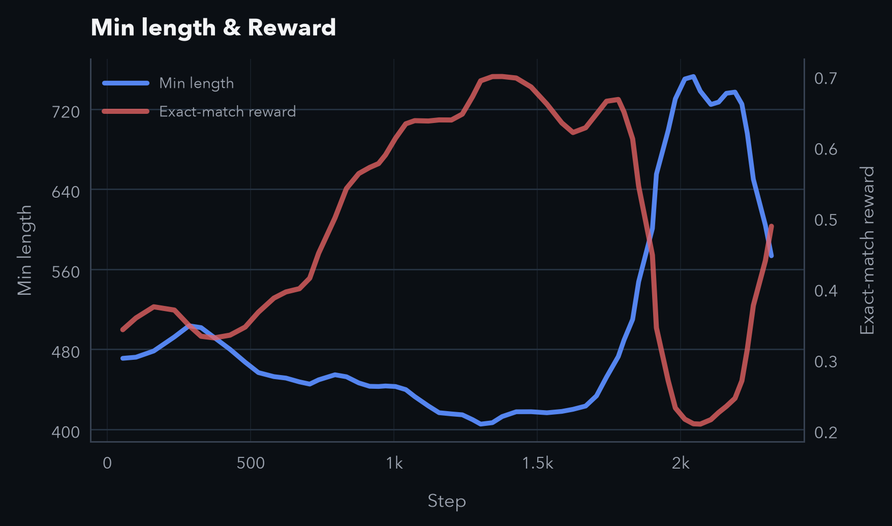
The model exploits the fact that it defines the points where a step potential is measured.
It tries to avoid ending a paragraph (outputting \n\n) unless the solution has become obvious.
If the reasoning first explores an incorrect strategy but then finds the correct way to the solution before ending the paragraph, it will receive a positive advantage since the paragraph made the solution more likely.
With a new line between those two strategies, the first and second attempts would receive separate, opposing feedback.
This pushes the policy towards long paragraphs at the cost of occasionally running into the token limit.
It is ironic that the policy tries to move back to outcome-level grading.
A pragmatic fix is very straightforward: introduce a max_paragraph_len (e.g. 128 tokens), after which a paragraph is split even without a newline.
These deliberately artificial splits (perhaps within a word, and very likely within a sentence) effectively enforce that paragraphs stay below this length.
With this guard the collapse was no longer observed and the training was more stable.
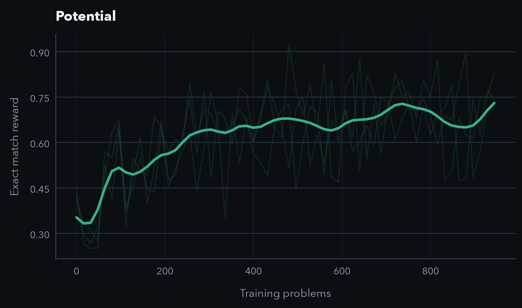
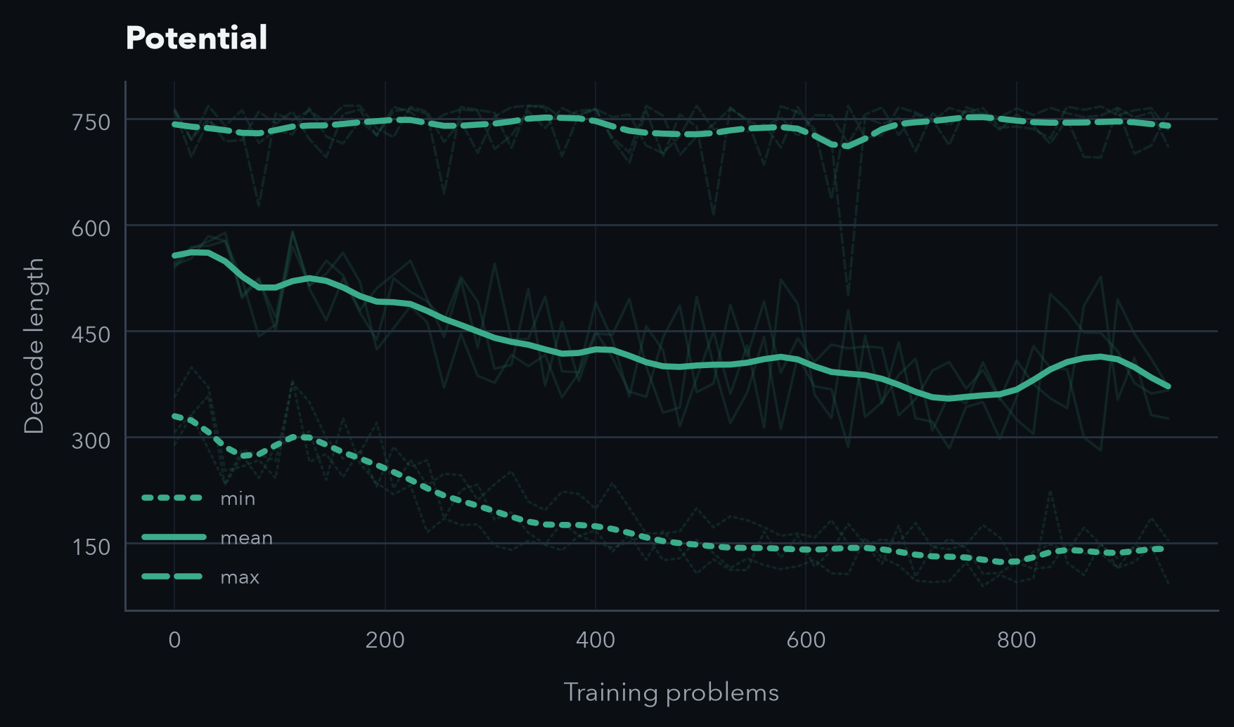
Results: promising start
The first set of experiments compares outcome-only RL with shaping with a frozen post-SFT scorer for up to 60 steps with three independent runs.
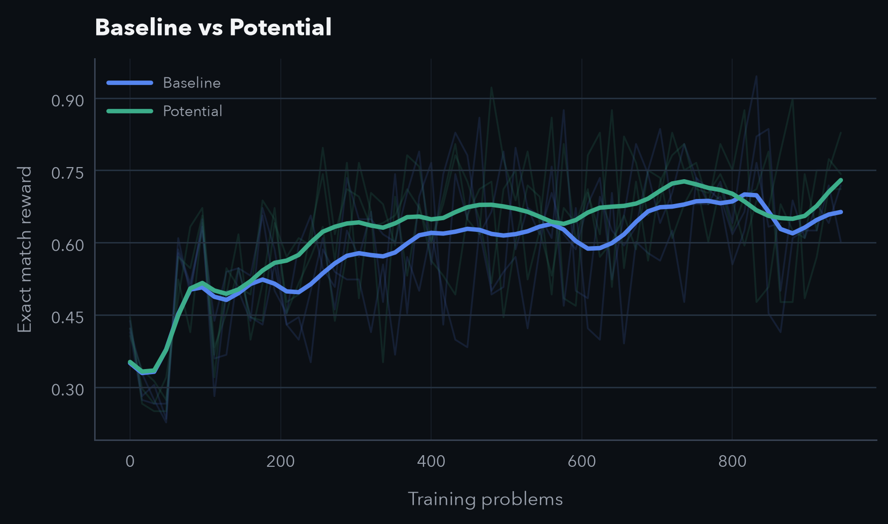
Evaluation uses 512 held-out puzzles, four samples per puzzle (so pass@4 might has high variance), temperature 0.8, and a maximum of 768 generated tokens (same as during training).
Besides comparing to the GRPO-style baseline, I also evaluated a non-contrastive potential estimation, that uses the provided ground-truth answer as a likelihood estimate.
| Method | Step 30 pass@1 / pass@4 | Step 60 pass@1 / pass@4 |
|---|---|---|
| Outcome-only baseline | 54.7 ± 0.4 / 64.9 ± 1.0 | 59.2 ± 0.8 / 70.7 ± 0.5 |
| Non-contrastive scorer | 55.5 ± 0.2 / 65.3 ± 1.8 | 59.6 ± 0.6 / 68.8 ± 4.1 |
| Frozen scorer | 60.7 ± 1.9 / 68.2 ± 1.2 | 62.3 ± 1.2 / 70.9 ± 1.5 |
That is a clear pass@1 improvement at both checkpoints compared to both the baseline and ablation. Pass@4 also improves at step 30, but is essentially tied by step 60.
This result is supported when we evaluate every five steps: our method quickly leads on pass@1 (after step 5) and maintains that lead through step 60. The short, early dip for pass@4 is not uncommon in RL settings. These methods are known for diversity-reducing behavior, increasing pass@1 performance at the cost of pass@k for k>1. MaxRL [17] and Poly-EPO [18] offer some elegant solutions to maintain explorative behavior.
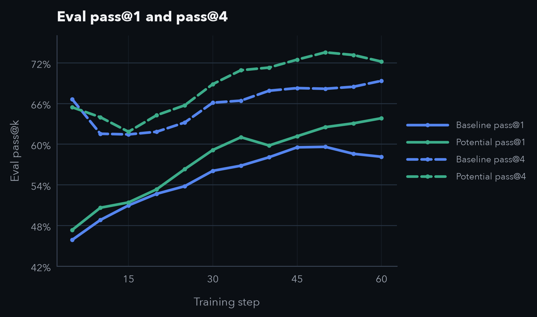
At this point, the method is clearly more sample-efficient than the baseline on pass@1.
Then I ran the same configurations for more steps, and the picture changed somewhat.
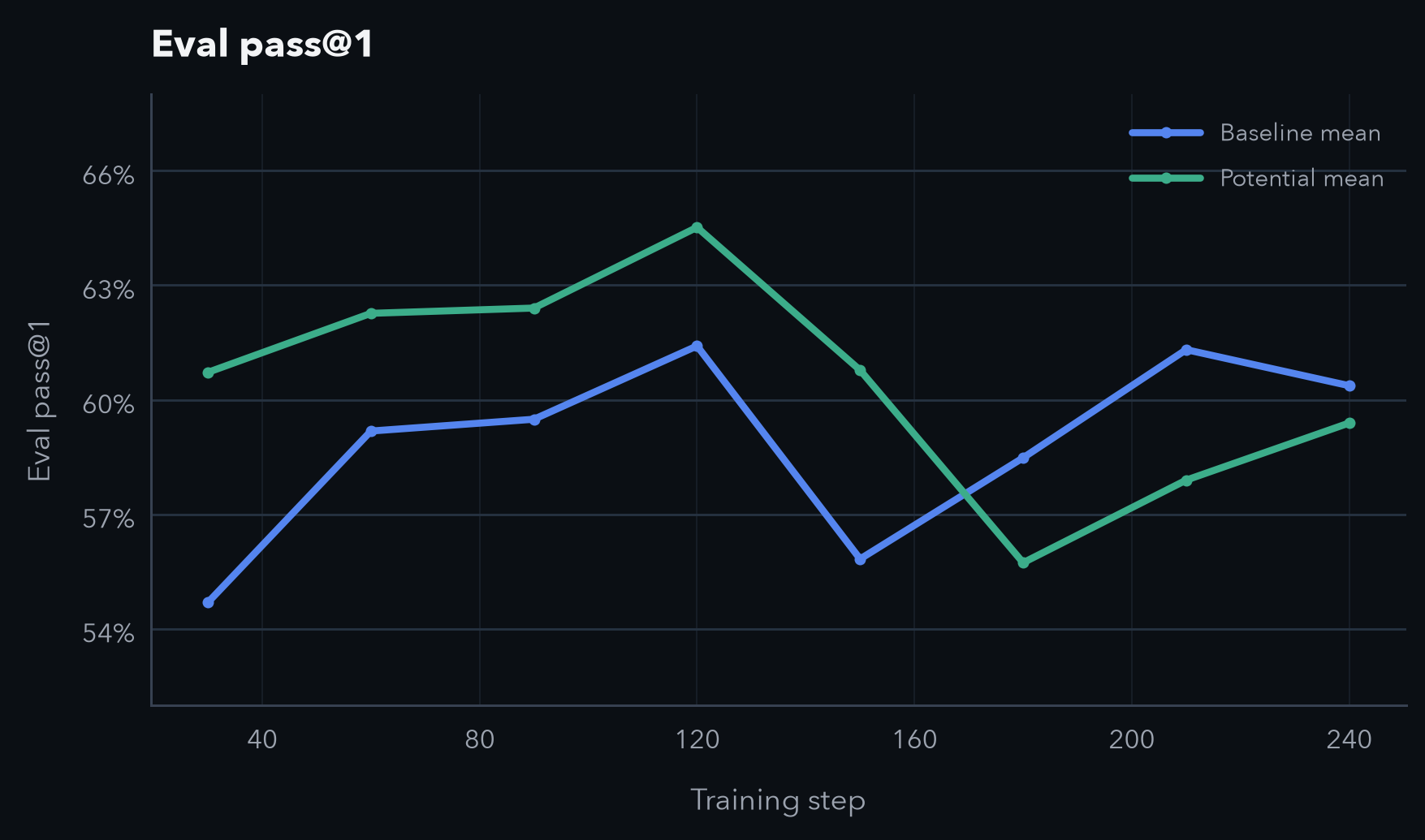
The faster early rise was still there (up until step 120), but the late-run performance of both methods was essentially the same. And while the potential-based method reached the highest performance at any point, it was later slightly less stable than the repeated baseline runs.
The natural next test was a moving scorer (the current policy), which removes the need to serve the post-SFT checkpoint on a separate vLLM server. I expected this to be the unstable configuration, but was surprised: it gave a very stable increase in reward, comparable to the constant post-SFT scorer.
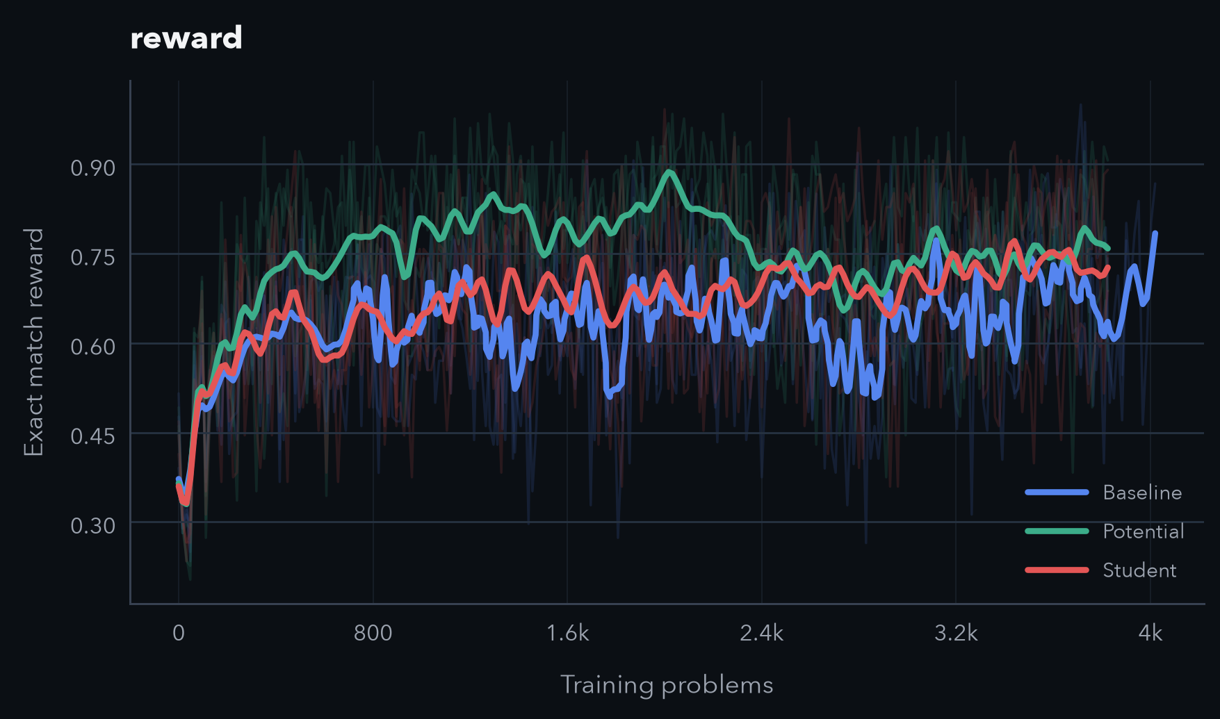
This is also reflected in the results:
| Method | Step 30 pass@1 / pass@4 | Step 60 pass@1 / pass@4 | Step 240 pass@1 / pass@4 |
|---|---|---|---|
| Outcome-only baseline | 54.7 ± 0.4 / 64.9 ± 1.0 | 59.2 ± 0.8 / 70.7 ± 0.5 | 60.4 ± 2.7 / 69.9 ± 3.3 |
| Frozen scorer | 60.7 ± 1.9 / 68.2 ± 1.2 | 62.3 ± 1.2 / 70.9 ± 1.5 | 59.4 ± 0.6 / 68.2 ± 0.8 |
| Moving scorer | 59.2 ± 2.4 / 69.2 ± 3.7 | 61.1 ± 0.9 / 70.0 ± 0.2 | 63.9 ± 1.0 / 75.1 ± 1.8 |
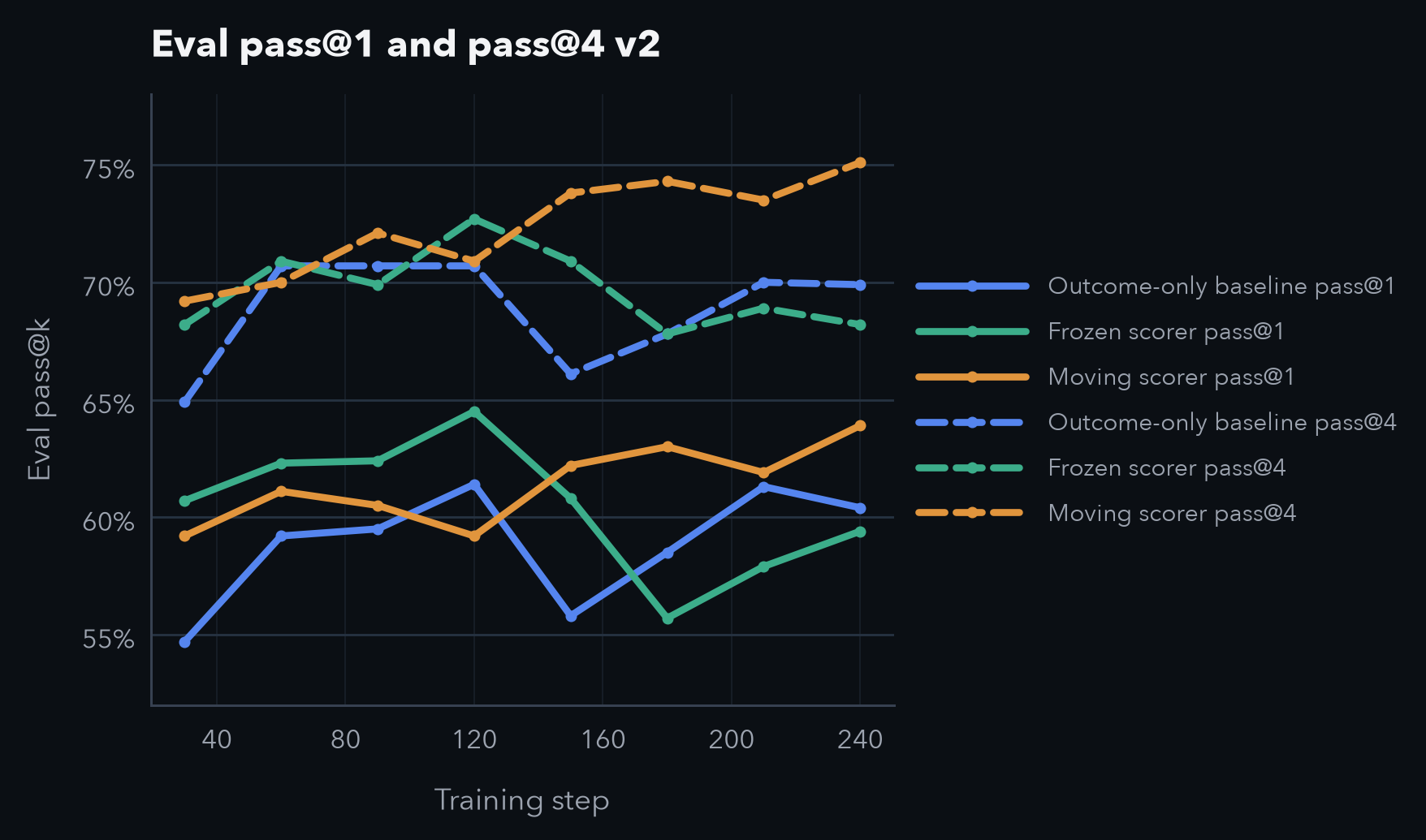
Both frozen and moving scorers gain an early pass@1 advantage over the baseline at step 30 and keep it at step 60. To assess later-stage performance and long-run stability, the moving-scorer runs are also evaluated after 240 steps. There they show the best performance across all checkpoints and methods, so they appear more stable and able to continue improving for longer.
The main conclusion is that contrastive step scoring improves early step efficiency, but with the frozen scorer it does not improve performance at the end of a very long run. For a moving scorer, we see slightly lower gains in early step efficiency, but more consistent and sustained training. Even after 240 optimization steps it does not seem to have reached a plateau and might improve further.
This is only a first exploration and demonstration of the method. These results obviously need further validation across different tasks and models, as well as comparison with other methods such as PRMs. However, I wanted to present it early to get feedback and be able to integrate it into the further development of the project. So please reach out via mail or on X and tell me what you like, didn't like, or if you want to collaborate.
Many projects and papers would end here, having successfully demonstrated an improved step-efficiency. That is fair, but not the whole picture. If one optimization step provides 2x the learning signal but takes 4x the time, it does not bring a practical benefit (GPUs are not rented per step). So let's have a look at a wall-time comparison.
vLLM improvements: Making the scorer (almost) free
The first implementation was substantially slower than the baseline (it took more than twice as long). At first glance this might not come as a surprise: we do compute a lot more. For each prompt, we sample eight rollouts and assume ten paragraphs each. For each truncated reasoning trace (80 in total), we score all eight candidate solutions (in the worst case; the answer bank is often smaller). That is 640 likelihood estimates per prompt, and with 16 prompts per batch, 10,240 likelihood calculations per gradient step.
That sounds like a lot. But is it?
Not as much as the count suggests, because these calculations are far from independent. Almost every sequence shares a long prefix with another: the untruncated reasoning trace is the only part we genuinely need to compute, and every truncation comes almost for free. The eight candidate answers all have the same prefix too. So far so good in theory, but let's have a look at what happens in practice.
Let's walk through the three implementation stages I went through.
First implementation (naive)
For a first proof-of-concept and some early experiments I used a very naive implementation. For every combination of
- rollout
- potential scoring point (paragraph end)
- answer candidate
in a batch, one scorer request was built and sent to vLLM's /inference/v1/generate endpoint with prompt_logprobs: 1 to receive logprobs for the whole sequence.
That works and is easy to verify, so it was good enough to start.
However, it carries several costs:
- one HTTP call per logical scoring request: not catastrophic, but pure overhead. We already know all scoring requests when we send the first.
- repeated work for duplicate requests: if two answers are identical, we don't need to score both, and we don't need to re-score the baseline (empty prefix) for every rollout, since it is shared.
- large responses: vLLM returned prompt-logprob structures for the whole sequence (as requested), but we only want the summed solution logprobs, so this is unnecessary transfer and parsing overhead.
As a quick-to-implement and easy-to-verify approach, this served its purpose, but scaling up the experiments required some optimizations.
Second implementation (obvious improvements)
Those costs are relatively easy to avoid with small changes:
- Deduplication of requests: saved roughly 12% of requests.
- A new batched endpoint: a new vLLM endpoint,
/inference/v1/prompt_logprobs, that accepts a batch of requests together with the target location (token indices of the solution) and returns just the summed logprob of the solution tokens per sequence instead of the full sequence logprobs. Sequences are still scheduled internally as before, with only the interface changing, which makes it easy to verify that outputs didn't change.
It is worth noting that logprob calculations are not bitwise-stable across batching and scheduling orders. I did see slight deviations between the batched implementation and the old reference, but they were the same magnitude as rerunning either implementation twice on the same sequence.
This improved the wall-clock time somewhat, but there was still a substantial overhead making any step-wise advantage practically useless. [3][3] Note that these are early runs with suboptimal hyperparameters, so their performance is different from the one reported above. ↩
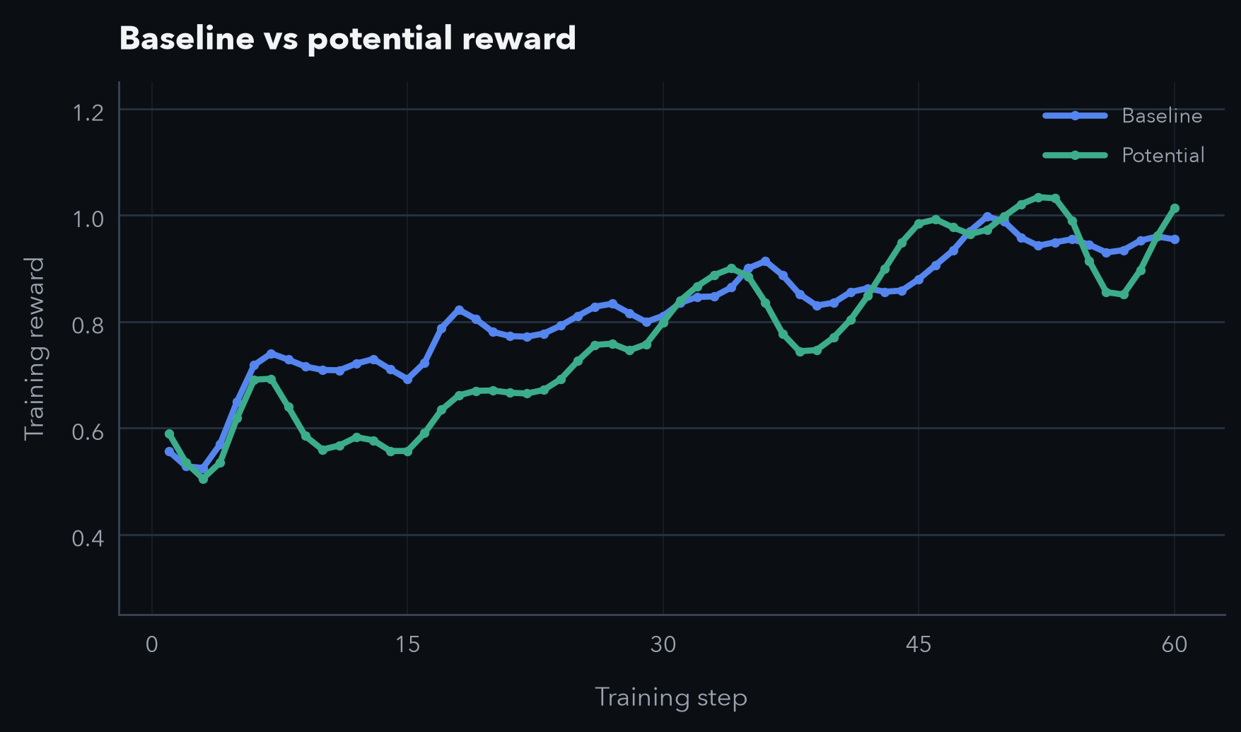
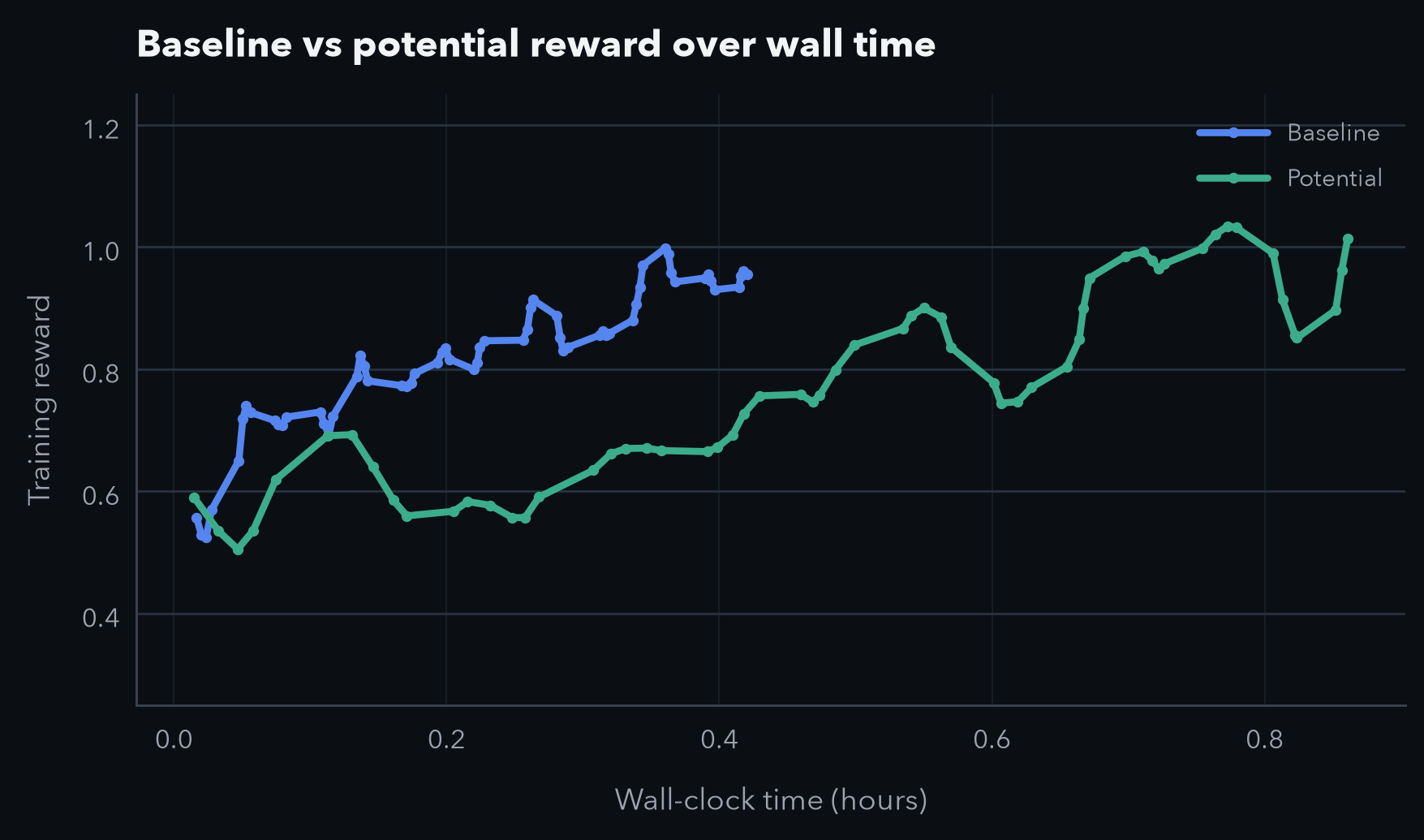
So is that all we can do? Not quite. The biggest optimization potential is still untapped, and it is a little hidden.
Usually vLLM does a great job at caching KV values, giving huge speed-ups over a naive recompute.
But for our scorer requests, it wasn't, as shown by prefix_cache_hits=0: every request recomputes the full sequence even though large parts are shared. Given that the truncated sequences are almost entirely contained in the untruncated one, vLLM should be reusing the cache. Why isn't it?
Third implementation (vLLM internals)
Once you see that every prefix is being recomputed, the opportunity is enormous: KV caching is the whole reason autoregressive generation is usable rather than prohibitively slow, and here we weren't using it at all.
The reason vLLM skips the cache here is justifiable. For generic prompt_logprobs requests it avoids serving any part of the prompt from the KV cache, because it does not recompute the logits for cached tokens and therefore cannot report their logprobs.
Rather than implementing a complex partial recomputation, vLLM simply disables prefix-cache reads for prompt_logprobs requests entirely. Sensible for the general API, but a major inefficiency for this use case.
We don't need logprobs for the whole prompt, only for the solution tokens, so everything before the solution (up to 99% of the sequence) can safely come from the cache.
Implementing this is straightforward: given a target_span, we manually allow prefix-cache reads up to the start of the target span (in practice, vLLM's block cache reads a few tokens less, but still the vast majority).
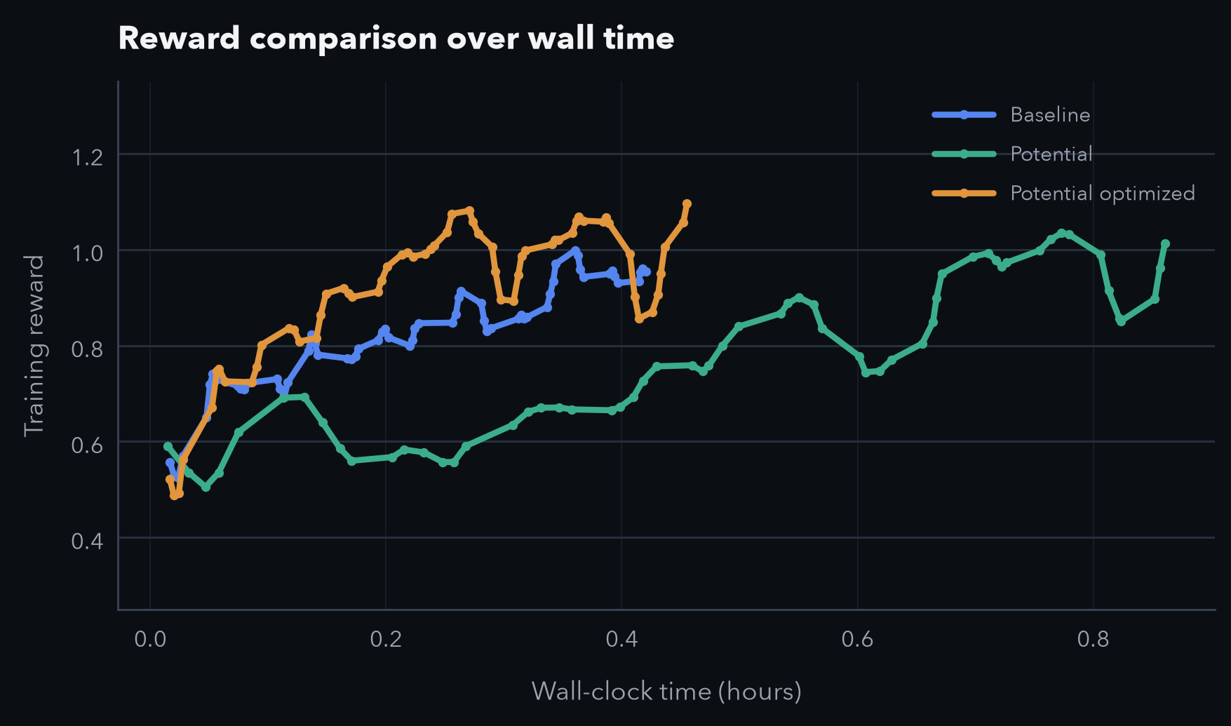
This was the main source of overhead. Without it, the cost of scoring all paragraphs is negligible compared to rollout generation. Now the early-step efficiency from earlier actually survives the conversion to wall-clock time, making the method a practical improvement.
Conclusion, limitations, and what's next
Two things came out of this. Methodologically, the contrastive answer-bank potential is a promising way to get a dense per-paragraph signal that is less sensitive to shared stylistic changes, and it does improve early-step efficiency. When using the same policy that is being optimized as the scorer, it also ends up with higher performance at step 240. On the systems side, the scorer that makes the method look expensive can be made nearly free by exploiting shared prefixes in the KV cache.
The project is far from complete. How does it behave with larger models? With more challenging tasks? With much longer reasoning traces or agentic setups, where credit assignment matters most? How to generalize to setups where scoring of an answer is non-trivial? Those are the directions I'm most curious about next. As mentioned earlier, feel free to reach out via mail or on X and tell me what you like, didn't like, or if you want to collaborate.
Further reading
- State of RL for reasoning LLMs: A comprehensive overview of GRPO and its improvements such as Dr. GRPO, DPPO, MaxRL, and more.
BibTeX
@misc{potential-2026,
  author = {Alexander Weers},
  title = {Denser rewards, nearly free: contrastive potential shaping},
  url = {https://aweers.de/blog/2026/potential/},
}
References
-
Fine-tuning language models from human preferences
arXiv preprint arXiv:1909.08593, 2019 ↩ -
Learning to summarize with human feedback
Advances in neural information processing systems, 2020 ↩ -
Training language models to follow instructions with human feedback
Advances in neural information processing systems, 2022 ↩ -
Let’s verify step by step
https://arxiv.org/abs/2305.20050, 2023 ↩ -
Scaling laws for reward model overoptimization
International Conference on Machine Learning, 2023 ↩ -
Policy invariance under reward transformations: Theory and application to reward shaping
Icml, 1999 ↩ -
Dynamic potential-based reward shaping
11th International Conference on Autonomous Agents and Multiagent Systems (AAMAS 2012), 2012 ↩ -
Dense reward for free in reinforcement learning from human feedback
arXiv preprint arXiv:2402.00782, 2024 ↩ -
PACR: Progressively Ascending Confidence Reward for LLM Reasoning
arXiv preprint arXiv:2510.22255, 2025 ↩ -
Tips: Turn-level information-potential reward shaping for search-augmented llms
arXiv preprint arXiv:2603.22293, 2026 ↩ -
Discovering Process-Outcome Credit in Multi-Step LLM Reasoning
arXiv preprint arXiv:2602.01034, 2026 ↩ -
Step Potential Advantage Estimation: Harnessing Intermediate Confidence and Correctness for Efficient Mathematical Reasoning
arXiv preprint arXiv:2601.03823, 2026 ↩ -
Well begun, half done: Reinforcement learning with prefix optimization for llm reasoning
Proceedings of the AAAI Conference on Artificial Intelligence, 2026 ↩ -
Vineppo: Refining credit assignment in rl training of llms
arXiv preprint arXiv:2410.01679, 2024 ↩ -
Math-shepherd: Verify and reinforce llms step-by-step without human annotations
Proceedings of the 62nd Annual Meeting of the Association for Computational Linguistics (Volume 1: Long Papers), 2024 ↩ -
DenseR: Dense Reward For Free in LLM Reasoning
2026 ↩ -
Maximum Likelihood Reinforcement Learning
2026 ↩ -
Poly-EPO: Training Exploratory Reasoning Models
arXiv preprint arXiv:2604.17654, 2026 ↩